Lecture 14

E12 Linear Physical Systems Analysis

Prof. Emad Masroor

March 5, 2026

Examples of second-order systems with damping

Second-order systems with damping

The second-order differential equation \[\ddot{x} + a \dot{x} + b x = 0\] usually has the solution \(x(t) =e^{s t}\) where \(s\) satisfies the characteristic equation \[s^2 + a s + b = 0 \implies s_{1,2} = \frac{-a \pm \sqrt{a^2-4b}}{2}\]

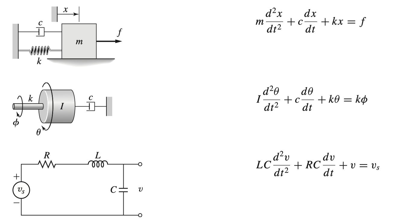
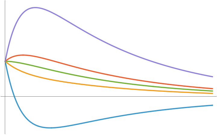
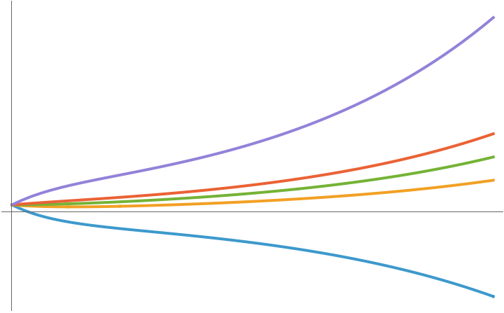
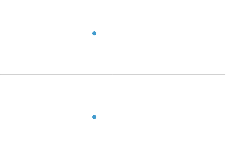
Case 1 when \(a^2 - 4b > 0\) and therefore \(s_{1,2} \in \mathbb{R}\)

\[x(t) = K_1 e^{s_1 t} + K_2 e^{s_2 t} \qquad K_1,K_2 \in \mathbb{R}\]

Case 1a: \(s_1,s_2 < 0\)	Case 1b: \(s_1< 0<s_2\)	Case 1c: \(s_1, s_2 > 0\)
Both roots negative	One positive, one negative	Both roots positive

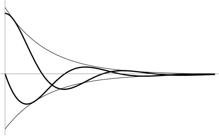
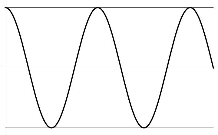
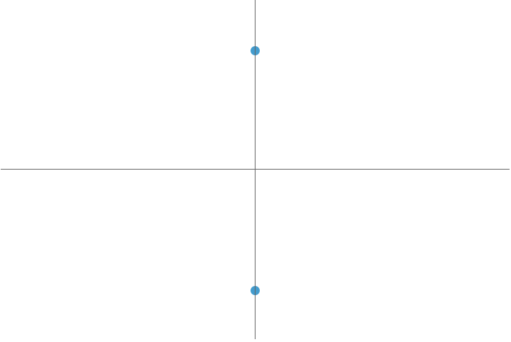
Case 2 when \(a^2 - 4b < 0\) and therefore \(s_{1,2} \in \mathbb{C}\)

\[ \begin{aligned} x(t) &= P e^{s_1 t} + \overline{P} e^{s_2 t} \qquad P \in \mathbb{C} \\ &= e^{rt} \left( A \cos \omega t + B \cos \omega t \right) \qquad A,B \in \mathbb{R} \\ s_{1,2} &= r \pm i \omega \end{aligned} \]

Case 2a: \(r < 0\)	Case 2b: \(r = 0\)	Case 2c: \(r > 0\)
Real part negative	Real part zero	Real part positive

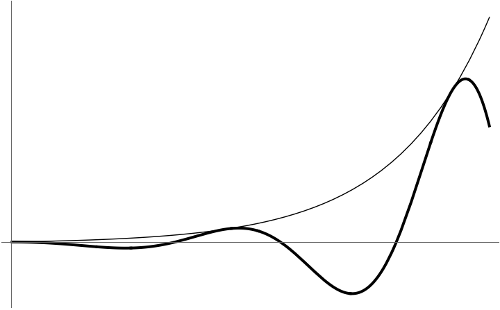
Case 3 when \(a^2 - 4b = 0\) and therefore \(s_1 = s_2\)

\[ x(t) = (C_1 + C_2t) e^{rt} \]

Case 3a: \(r < 0\)	Case 3b: \(r = 0\)
Nonzero repeated roots	Repeated roots at zero

Summary of 2nd-order systems with no input

The differential equation \[m \ddot{x} + b \dot{x} + k x = 0\]

admits solutions of the form \(e^{st}\) where \(s\) must be a root of the characteristic polynomial \[m s^2 + b s + k.\] The roots will, in general, be complex, and are given by \[s_{1,2} = \frac{-b \pm \sqrt{b^2-4mk}}{2m}.\] Then, the solution can usually be written as \[x(t) = A e^{s_1t} + B e^{s_2 t}\] where \(A\) and \(B\) are, in general, complex.

Case 1: Roots of characteristic polynomial are real

If \(b^2-4mk >0\), the two roots are real and are given by the real numbers \[s_{1,2} = \frac{-b \pm \sqrt{b^2-4mk}}{2m}\] and the solution can be written as \[\boxed{x(t) = K_1 e^{s_1 t} + K_2 e^{s_2 t}} \qquad \text{with }K_1,K_2,s_1,s_2 \in \mathbb{R}\]

Case 2: Roots of characteristic polynomial are complex

If \(b^2-4mk <0\), the two roots are complex and are given by the complex numbers \[ s_{1,2} = \frac{-b \pm \sqrt{b^2-4mk}}{2m} = r \pm i \omega, \] \[ \text{ where } \quad r = -\frac{b}{2m}, \quad \omega = \frac{1}{2m}\sqrt{4mk-b^2}\] and the solution can be written as \[x(t) = P e^{s_1 t} + \overline{P} e^{s_2 t} \qquad \text{with }P,s_1,s_2 \in \mathbb{C}\] or, alternatively, as \[\boxed{x(t) = e^{rt} \left( K_3 \cos \omega t + K_4 \sin \omega t \right)} \qquad \text{with }K_3,K_4,r,\omega \in \mathbb{R}\] or, alternatively, as \[x(t) = e^{rt} C_1 \cos \left( \omega t + \phi_1 \right) \qquad \text{with }C_1,\phi_1,r,\omega \in \mathbb{R}\] or, alternatively, as \[x(t) = e^{rt} C_2 \sin \left( \omega t + \phi_2 \right) \qquad \text{with }C_2,\phi_2,r,\omega \in \mathbb{R}\]

Case 3: Roots of characteristic polynomial are repeated

If \(b^2-4mk =0\), the two roots are repeated \[ s_1 = s_2 = \frac{-b \pm \sqrt{{b^2-4mk}}}{2m} = -b/2m = r\] and the solution can be written as (take MATH 43/44 to see why) \[\boxed{x(t) = (C_3 + C_4t) e^{rt}} \qquad \text{with }C_3,C_4,r \in \mathbb{R}\]

Changing the damping

Let’s examine solutions to \[m \ddot{x} + b \dot{x} + k x = 0, \qquad x(0) = 1, \dot{x}(0) = 0\] With \(k=2\), \(m=3\), and \(b\) allowed to vary from \(0\) to \(6\).

Value of \(b\)	Motion
\(0.0\)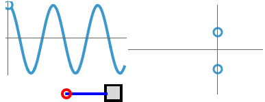
\(0.5\)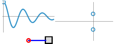
\(1.0\)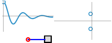
\(1.5\)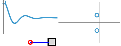
\(2.0\)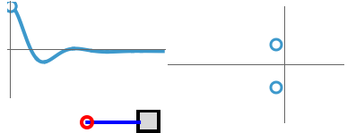
\(2.5\)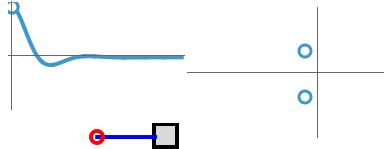
\(3.0\)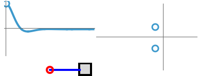
\(3.5\)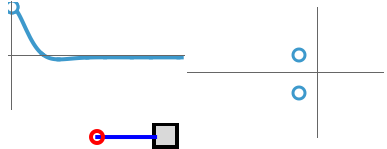
\(4.0\)
\(4.5\)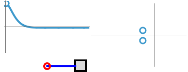
\(5.0\)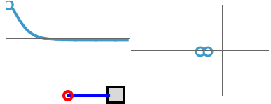
\(5.5\)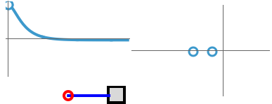
\(6.0\)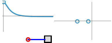

Effect of Root Location on free response

The system \(m \ddot{x} + b \dot{x} + kx = f(t)\) has a free response that depends on the roots of the characteristic polynomial \(m s^2 + b s + k\).

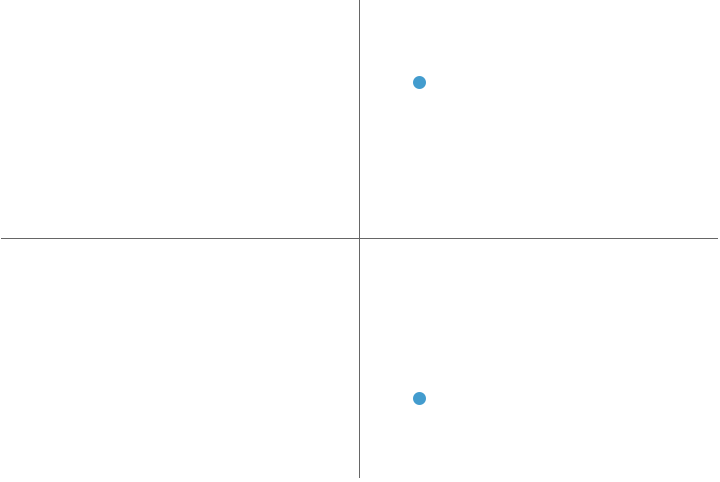
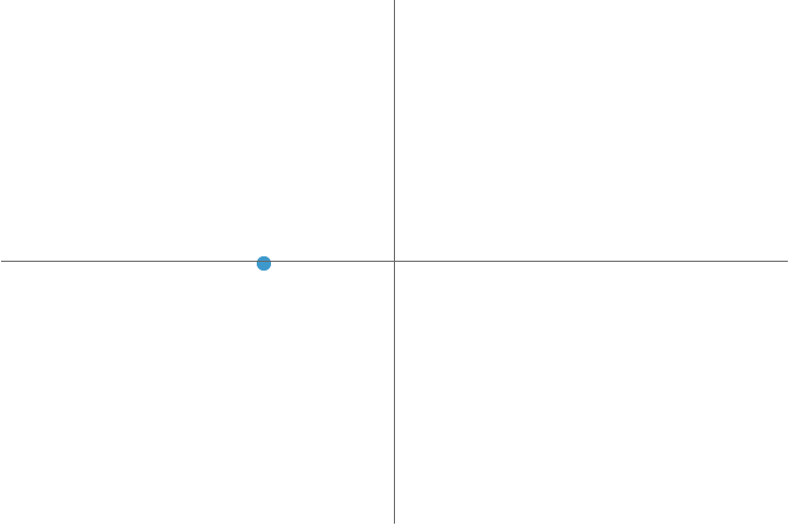
In general, these roots are complex, so we can plot them on the complex plane.

Note: This diagram from Palm, System Dynamics uses \(j\) for the imaginary unit instead of \(i\).

Critical Value of Damping

We’ve seen that something special happens when the damping coefficient \(b\) crosses some critical value. What is this critical value?

\(m \ddot{x} + b \dot{x} + kx = 0\) has the solutions \(e^{st}\) when \[m s^2 + b s + k = 0 \implies s = \frac{-b \pm \sqrt{b^2-4mk}}{2m}\]

• If \(b^2 - 4mk < 0\): \(\quad s_{1,2}\) has nonzero imaginary part (\(s_{1,2} \in \mathbb{C}\))
• If \(b^2 - 4mk > 0\): \(\quad s_{1,2}\) has zero imaginary part (\(s_{1,2} \in \mathbb{R}\))
• If \(b^2 - 4mk = 0\): \(\quad s_1 = s_2\) (repeated nonzero roots)

Recall that if — and only if — \(s \in \mathbb{C}\), then \(e^{st}\) will oscillate in time! (\(e^{i\theta} = \cos \theta + ...\))

There is a critical value of \(b = \sqrt{4mk}\) that demarcates qualitatively different behavior.

Introducing Damping Ratio

• There is a critical value of \(b = \sqrt{4mk}\) that demarcates qualitatively different behavior.
• Define a ratio \(\zeta\) (Greek letter ‘zeta’) \[\zeta = \frac{b}{\sqrt{4mk}}\] that is the ratio of damping parameter \(b\) to the critical damping parameter

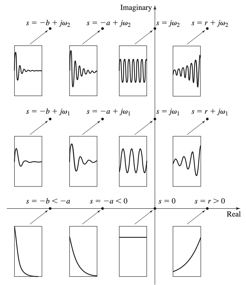
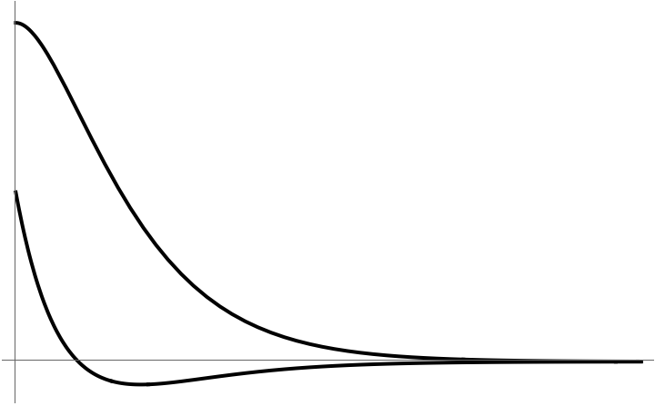
Underdamped, overdamped, etc.

Zeta \(\zeta\)	\(b\)	Name	Typical Motion and roots of \(m s^2 + b s + k\)
\(\zeta = 0\)	\(b=0\)	Undamped
\(\zeta < 1\)	\(b < \sqrt{4mk}\)	Underdamped
\(\zeta = 1\)	\(b = \sqrt{4mk}\)	Critically damped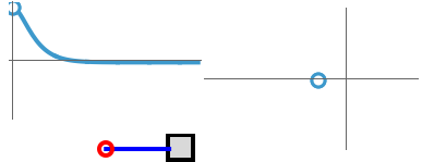
\(\zeta > 1\)	\(b > \sqrt{4mk}\)	Overdamped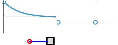

Governing equation for 2nd order system in terms of natural freqency and damping ratio

Recall that the natural frequency is given by \(\sqrt{k/m}\). From now on, we will call this the ‘undamped natural frequency’ and use the symbol \(\boxed{\omega_n}\).

\[ m \ddot{x} + b \dot{x} + kx = 0 \] \[ \phantom{m} \ddot{x} + \frac{b}{m} \dot{x} + \frac{k}{m}x = 0 \] \[ \phantom{m} \ddot{x} + \overbrace{\frac{{\color{green}{b}}}{m} \cdot \frac{\sqrt{m}}{{\color{green}{\sqrt{m}}}} \cdot \frac{\sqrt{k}}{{\color{green}{\sqrt{k}}}} \cdot \frac{2}{{\color{green}{2}}}}^{b/m} \dot{x} + \left(\frac{\sqrt{k}}{\sqrt{m}}\right)^2 x = 0 \] \[ \phantom{m} \ddot{x} + \frac{{\color{green}{b}}}{{\color{brown}{\sqrt{m}}}} \cdot \frac{{1}}{{\color{green}{\sqrt{m}}}} \cdot \frac{{\color{brown}{\sqrt{k}}}}{{\color{green}{\sqrt{k}}}} \cdot \frac{2}{{\color{green}{2}}} \dot{x} + \left(\frac{{\color{brown}{\sqrt{k}}}}{{\color{brown}{\sqrt{m}}}}\right)^2 x = 0 \] \[ {\color{green}{\frac{b}{2\sqrt{mk}}}} \text{ is the damping ratio } \zeta \] \[ {\color{brown}{\sqrt{\frac{k}{m}}}} \text{ is the undamped natural frequency } \omega_n \] \[ \implies \boxed{\ddot{x} + 2 {\color{green}{\zeta}}{\color{brown}{\omega_n}} x + {\color{brown}{\omega^2_n}} x = 0} \]

Damped vs. undamped natural frequency

We know that a system governed by \(m \ddot{x} + kx = 0\) has the free response \[ \begin{aligned} \textstyle x(t) &= \textstyle A \cos \left( t \sqrt{k/m} \right) + B \sin \left( t \sqrt{k/m} \right) \\ &= A \cos \omega_n t + B \sin \omega_n t \end{aligned} \] where \(A, B \in \mathbb{R}\) can be found using the initial conditions.

At what frequency does the system governed by \[m \ddot{x} + b \dot{x} + kx = 0 \tag{1}\] oscillate naturally?

1. Same as \(\omega_n\) ?
2. Faster than the undamped system?
3. Slower than the undamped system?

Hint: Equation 1 is identical to \(\ddot{x} + 2 \zeta \omega_n x + \omega_n^2 x = 0\)

Damped Natural Frequency and Time Constant for second-order systems

Underdamped second order systems (with \(\zeta < 1\)) have a time constant that characterizes how quickly or slowly they decay.

Solutions are multiples of \(x(t) = e^{({\color{blue}{r}} \pm i {\color{brown}{\omega}} )t}\).

• \({\color{brown}{\omega}}\) is responsible for the oscillation
• \({\color{blue}{r}}\) is responsible for the decay

When \(m \ddot{x} + b \dot{x} + k x = 0\) is written in the form \[\ddot{x} + 2 \zeta \omega_n x + \omega_n^2 x = 0,\]

the roots of the characteristic polynomial \[s^2 + 2 \zeta \omega_n s + \omega_n^2\] are \[s = - \zeta \omega_n \pm i \omega_n \sqrt{1-\zeta^2}\]

with the solution for \(x(t)\) given by \[x(t) = e^{- {\color{blue}{\zeta \omega_n}}t} \left( A \cos \left( t\, {\color{brown}{\omega_n \sqrt{1-\zeta^2}}} \right) + B \sin \left( t\, {\color{brown}{\omega_n \sqrt{1-\zeta^2}}} \right) \right)\]

• \(\displaystyle {\color{blue}{\frac{1}{\zeta \omega_n}}}\) is known as the time constant
• \({\color{brown}{\omega_n \sqrt{1-\zeta^2}}}\) is known as the damped natural frequency

Step Response of a second-order system

Consider a spring-mass system starting from \(x = 0, \dot{x}=0\) that is subjected to a step function force \(f(t) = u_s(t)\)

\[\ddot{x} + 2 \zeta \omega_n \dot{x} + \omega_n^2 x = u_s(t)\]

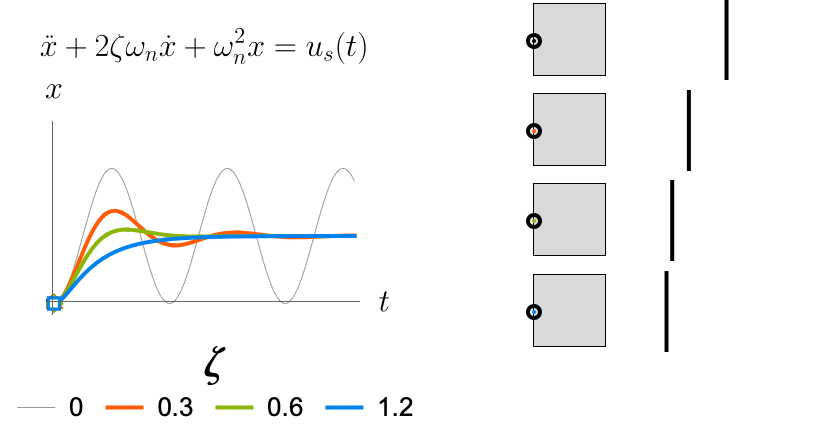
• When \(\zeta < 1\), overshoot occurs
• When \(\zeta > 1\), there’s no overshoot

Calculating the step response of a second-order system

Q. How does a spring-mass-damper system respond to a step-function force applied to it?

Approach:

1. Write the differential equation
2. Take Laplace Transform
3. Solve for \(X(s)\)
4. Use Inverse Laplace Transform to get \(x(t)\)

\[ m \ddot{x} + b \dot{x} + k x = u_s(t) \] \[ \mathcal{L}\left[ m \ddot{x} + b \dot{x} + k x \right] = \mathcal{L} \left[ u_s(t) \right] \] \[ m s^2 X + b s X + k X = \frac{1}{s} \] \[ \left( m s^2 + b s + k \right) X = \frac{1}{s} \] \[ X(s) = \frac{1}{s} \frac{1}{ m s^2 + b s + k} \]

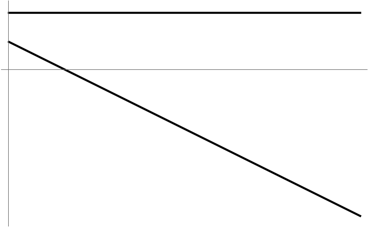
Impulse Response of a second-order system

Consider a spring-mass system starting from \(x = 0, \dot{x}=0\) that is subjected to a impulse function force \(f(t) = \delta(t)\)

\[\ddot{x} + 2 \zeta \omega_n \dot{x} + \omega_n^2 x = \delta(t)\]

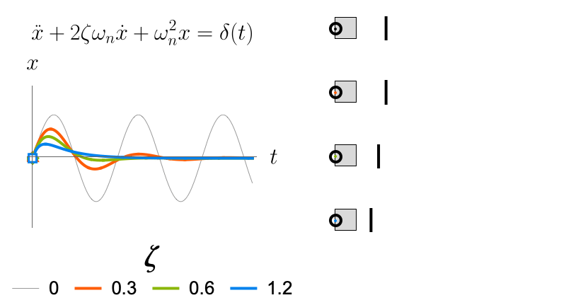
• When \(\zeta > 1\), no oscillations occur
• When \(\zeta < 1\), there’s oscillations

Calculating the impulse response of a second-order system

Q. How does a spring-mass-damper system respond to a Dirac Delta-function force applied to it?

Approach:

1. Write the differential equation
2. Take Laplace Transform
3. Solve for \(X(s)\)
4. Use Inverse Laplace Transform to get \(x(t)\)

\[ m \ddot{x} + b \dot{x} + k x = \delta(t) \] \[ \mathcal{L}\left[ m \ddot{x} + b \dot{x} + k x \right] = \mathcal{L} \left[ \delta(t) \right] \] \[ m s^2 X + b s X + k X = 1 \] \[ \left( m s^2 + b s + k \right) X = 1 \] \[ X(s) = \frac{1}{ m s^2 + b s + k} \]