Lecture 17
E12 Linear Physical Systems Analysis
March 24, 2026
Free and Forced Response of linear systems
Recall that the free and forced response can be determined with the help of the Laplace Transform.
\[m \ddot{x} + b \dot{x} + k x = f(t)\]
\[\mathcal{L}[m \ddot{x} + b \dot{x} + k x ]= \mathcal{L}[f(t)]\]
\[\mathcal{L}[m \ddot{x}] + \mathcal{L}[b \dot{x}] + \mathcal{L}[k x ]= F(s)\]
\[
\begin{aligned}
\mathcal{L}[m \ddot{x}(t)] &= m \left( s^2 X(s) - s x(0) - \dot{x}(0) \right) \\
\mathcal{L}[b \dot{x}(t)] &= b \left( s X(s) - x(0) \right) \\
\mathcal{L}[k x(t)] &= k X(s)
\end{aligned}
\]
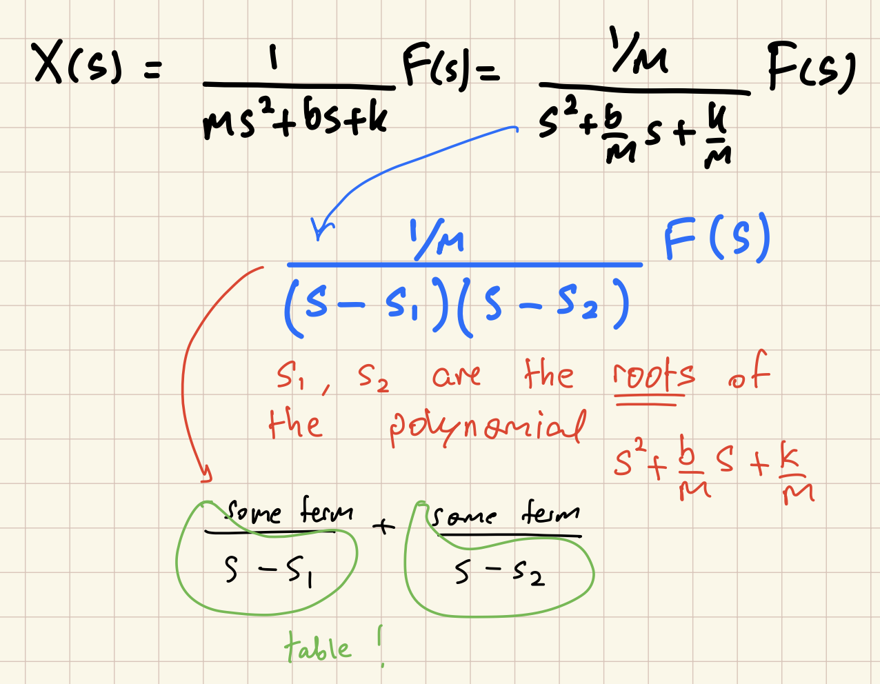
Rearrange to get \(X(s)\) in terms of the sum of two terms:
- A term dependent on \(F(s)\), and
- A term dependent on \(x(0)\) and \(\dot{x}(0)\).
Free and Forced Response of 2nd-order systems
\[
X(s) = \frac{1}{m s^2 + b s + k} F(s) + \frac{x(0) (ms + b) + m\dot{x}(0)}{m s^2 + b s + k}
\]
\[
\begin{aligned}
X(s) &= \frac{1}{m s^2 + b s + k} F(s) \\
&+ \frac{(ms + b)}{m s^2 + b s + k} x(0) \\
&+ \frac{m}{m s^2 + b s + k} \dot{x}(0)
\end{aligned}
\]
- A term that depends on \(\mathcal{L}[f(t)]\)
- A term that depends on \(x(0)\)
- A term that depends on \(\dot{x}(0)\)
The Transfer Function and the Forced Response
The Transfer Function encodes the linear relationship between the input (a.k.a forcing function) and output (a.k.a. forced response) of a linear system.
\[
\begin{aligned}
m \ddot{x} + b \dot{x} + k x &= f(t) \\
X(s) &= \frac{1}{m s^2 + b s + k} F(s) \\
X(s) &= T(s) F(s)
\end{aligned}
\]
Free, Forced, Transient, Steady-State
- Free response: The part of the response that depends on the initial conditions
- Forced response: The part of the response that is due to the forcing function
- Transient Response: The part of the response that disappears at long times
- Steady-State Response: The part of the response that remains at long times.
Calculating Free, Forced, Transient, Steady
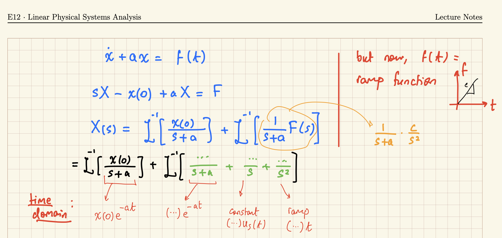
Show that the transient and steady-state parts of the response of a system \[\dot{x} + ax = f(t)\] to a ramp input \(f(t) = ct\) is \[\underbrace{x(0) e^{-at} + \frac{c}{a^2} e^{-at}}_{\text{transient}} + \underbrace{\frac{c}{a} t - \frac{c}{a^2}}_{\text{steady state}}\]
![]()
Stability
- Unstable: A system is unstable if its free response approaches \(\pm \infty\) as \(t \rightarrow \infty\)
- Stable: A system is stable if its free response approaches \(0\) as \(t \rightarrow \infty\)
- Neutrally Stable: A system is neutrally stable if its free response neither approaches \(\pm \infty\) nor approachs \(0\) as \(t \rightarrow \infty\).
- Stability is a property of a system, and does not depend on what input is paplied to the system.
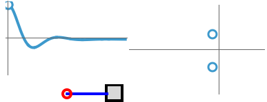
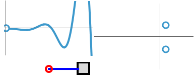
Stability and the roots of the characteristic polynomial
![]()
![]()
- Unstable behavior occurs when the root lies to the right of the imaginary axis.
- Neutrally stable behavior occurs when the root lies on the imaginary axis.
- The response oscillates only when the root has a nonzero imaginary part.
- The greater the imaginary part, the higher the frequency of the oscillation.
- The farther to the left the root lies, the faster the response decays.
The Transfer Function can represent a system’s equations
A linear system can be represented either as a set of differential equations or as a transfer function.
Differential Equation
\[\ddot{x} + 5 \dot{x} + 7 x = f(t)\]
Transfer Function
\[X(s) = \frac{1}{s^2 + 5s + 7} F(s)\]
- Sometimes, systems are specified using just their transfer function.
- Given a transfer fucntion \(T(s)\), it is assumed that we are referring to an equation of the form \(X(s) = T(s) F(s)\).
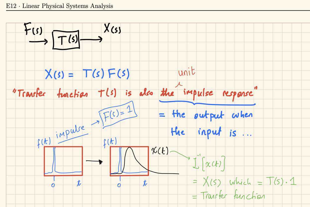
The Transfer Function is also the impulse response
For any linear system, its transfer function is also its impulse response.
- What does this mean?
- Why is this true?
Equivalent Representations
The following information is equivalent, and any one of hte following fully specifies a linear system.
| Differential Equation |
\(\ddot{x} + 5 \dot{x} + 7 x = f(t)\) |
| Transfer Function |
\(\displaystyle \frac{1}{s^2 + 5s + 7}\) |
| Characteristic Polynomial |
\(s^2 + 5s + 7\) |
| Characteristic Equation |
\(s^2 + 5s + 7 = 0\) |
| Roots (of the characteristic polynomial) |
\(s = \displaystyle \frac{1}{2} \left( -5 \pm i \sqrt{3} \right)\) |
| Impulse Response |
\(\displaystyle \frac{2}{\sqrt{3}} e^{-5 t/2} \sin \left(\frac{\sqrt{3} t}{2}\right)\) |
Transfer Functions as rational functions of \(s\)
Recall that a rational function of \(s\) is a ratio \[\frac{P(s)}{Q(s)}\]
where \(P(s)\) is a polynomial of degree \(m\) and \(Q(s)\) is a polynomial of degree \(n\).
In E12, we will always have \(m < n\)
- Recall that any polynomial of degree \(n\) is fully defined by a set of \(n+1\) coefficients
- In E12, our polynomials will always have real coefficients.
- If \(P(s)\) has degree \(>0\), then the system is said to have numerator dynamics
- Typically, this happens when the output depends on derivatives of the input
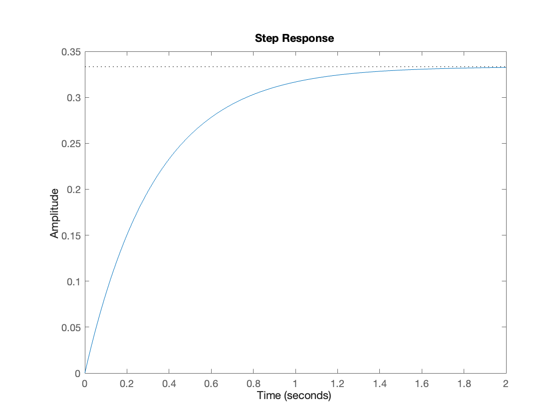
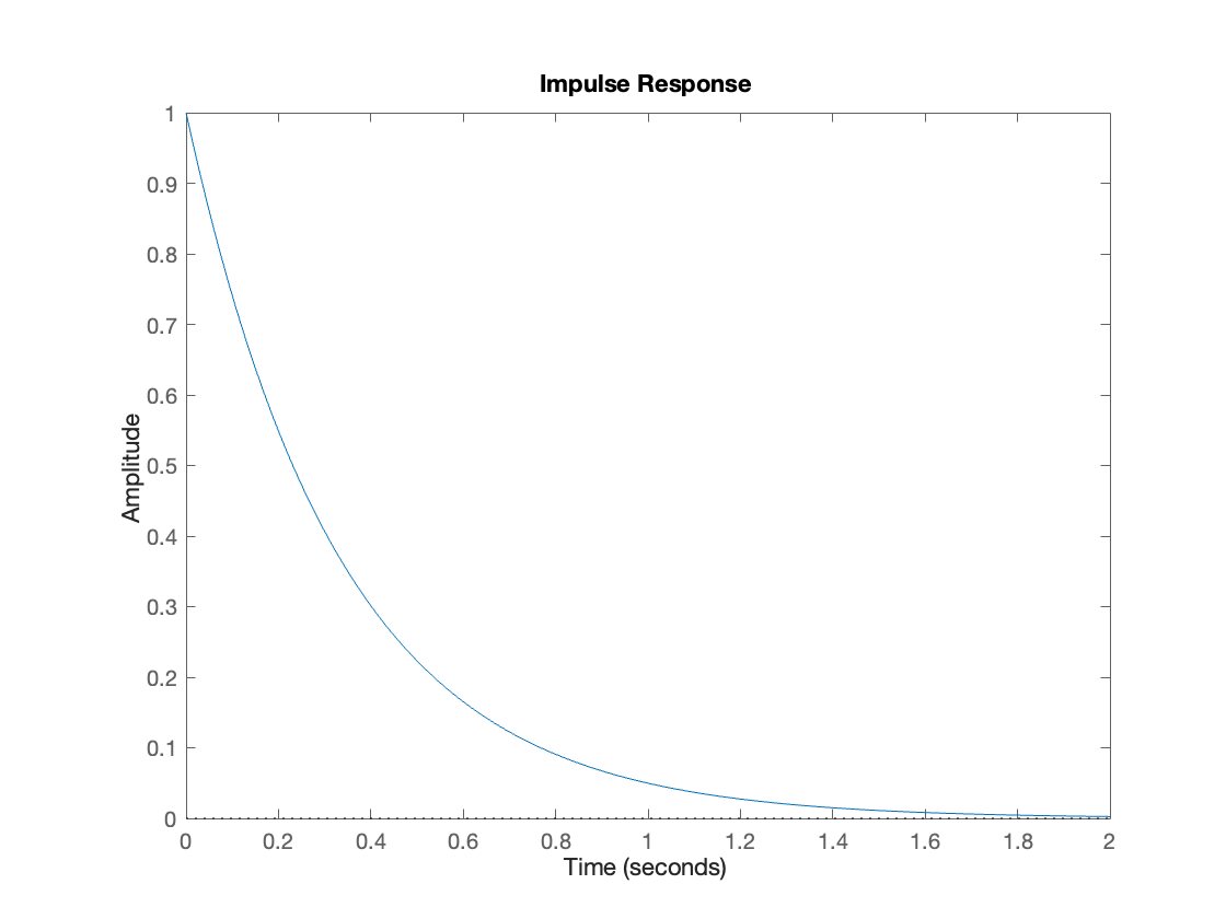
Create some tf objects in MATLAB
- Create the system
- Examine its impulse response
- Examine its step response
For the following systems:
- \(T(s) = \frac{1}{s+3}\)
- \(T(s) = \frac{1}{2s+3}\)
- \(T(s) = \frac{1}{s-3}\)
- \(T(s) = \frac{1}{s^2+5s+7}\)