Lecture 18
E12 Linear Physical Systems Analysis
March 26, 2026
Forced Response of 1st order systems
\[\dot{x} + ax = f(t)\]
| Input | \(f(t)\) | \(F(s)\) | Response \(X(s)\) | Response \(x(t)\) |
|---|---|---|---|---|
Step  |
\(b u_s(t)\) | \(\displaystyle \frac{b}{s}\) | \(\displaystyle \frac{b}{s} \frac{1}{s+a}\) | \(\displaystyle \frac{b}{a} \left( 1 - e^{-at} \right)\) 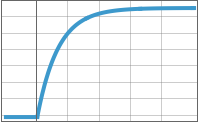 |
Impulse  |
\(A \delta(t)\) | \(A\) | \(A \displaystyle\frac{1}{s+a}\) | \(\displaystyle A e^{-at} \phantom{\left( 1 - e^{-at} \right)}\) 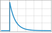 |
Ramp 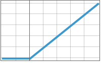 |
\(u_s(t) \cdot c t\) | \(\displaystyle \frac{c}{s^2}\) | \(\displaystyle \frac{c}{s^2} \frac{1}{s+a}\) | \(\displaystyle \frac{c}{a^2} \left( e^{-at} - 1\right) + \frac{c}{a} t\) 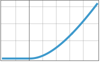 |
Sinusoid  |
\(u_s(t) \cdot \sin \omega t\) | \(\displaystyle \frac{\omega}{s^2+\omega^2}\) | \(\displaystyle \frac{\omega}{s^2+\omega^2} \frac{1}{s+a}\) | \(\displaystyle \phantom{\frac{c}{a^2} \left( e^{-at} - 1\right) + \frac{c}{a} t}\) 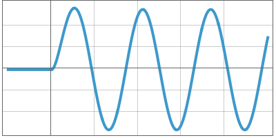 |
What about second-order systems?
\[m \ddot{x} + b \dot{x} + kx = f(t)\]
| Input | \(f(t)\) | \(F(s)\) | Response \(X(s)\) | Response \(x(t)\) |
|---|---|---|---|---|
Step  |
\(b u_s(t)\) | \(\displaystyle \frac{b}{s}\) | \(\displaystyle \frac{b}{s} \frac{1}{ms^2 + b s + k}\) | \(\displaystyle \phantom{\frac{b}{a} \left( 1 - e^{-at} \right)}\) |
Impulse 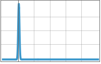 |
\(A \delta(t)\) | \(A\) | \(A \displaystyle \frac{1}{ms^2 + b s + k}\) | |
Ramp 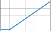 |
\(u_s(t) \cdot c t\) | \(\displaystyle \frac{c}{s^2}\) | \(\displaystyle \frac{c}{s^2} \frac{1}{ms^2 + b s + k}\) | |
Sinusoid 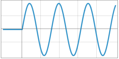 |
\(u_s(t) \cdot \sin \omega t\) | \(\displaystyle \frac{\omega}{s^2+\omega^2}\) | \(\displaystyle \frac{\omega}{s^2+\omega^2} \frac{1}{m s^2 + bs + k}\) |
Standard Form of a second-order linear system

Practice
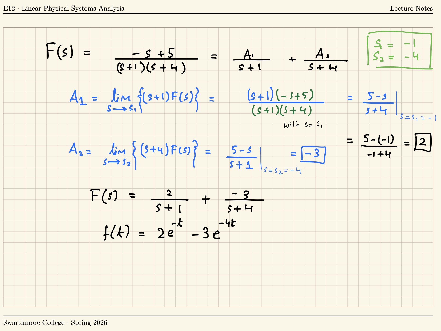
Find the inverse Laplace Transform of the following function: \[F(s) = \frac{5-s}{s^2 + 5s + 4}\]
Practice
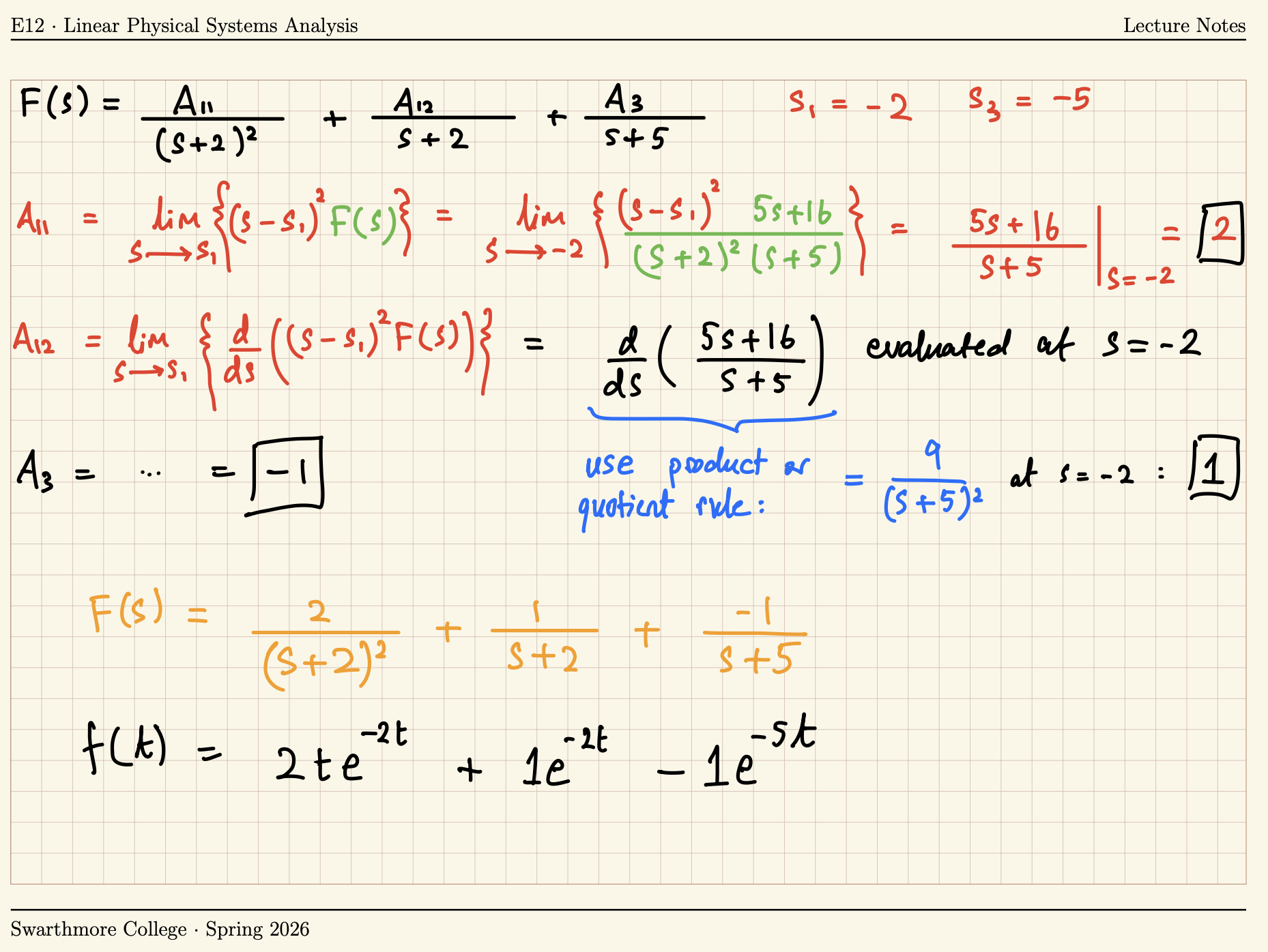
Find the inverse Laplace Transform of the following function: \[F(s) = \frac{5s+16}{(s+2)^2 (s+5)}\]
Partial Fractions Expansion for Complex Poles
Consider \[F(s) = \frac{N(s)}{D(s)}\] where \(D(s)\) has two complex roots.
Then \[F(s) = \frac{Bs+C}{(s-(r+i\omega))(s-(r-i\omega))}\]
- It is possible to re-write \(F(s)\) as \[F(s) = \frac{K_1}{s-(r+i\omega)} + \frac{K_2}{s-(r-i\omega)}\]
- but \(K_1\) and \(K_2\) will have to be complex.
- We can apply the formula for the distinct-pole coefficients \(K_1\) and \(K_2\), i.e. \[ \begin{aligned} K_1 &= \lim_{s \rightarrow r+i\omega} \left[ (s-(r+i\omega))F(s) \right] \\ K_2 &= \lim_{s \rightarrow r-i\omega} \left[ (s-(r-i\omega))F(s) \right] \end{aligned} \]
- and this shows us that \(K_1\) and \(K_2\) are complex conjugates of each other.
- Thus, \[F(s) = \frac{K e^{i \phi}}{s-(r+i\omega)} + \frac{K e^{-i\phi}}{s-(r-i\omega)}\]
- which can be transformed back into the time domain as \[f(t) = Ke^{i \phi} e^{(r+i\omega)t} + Ke^{-i \phi} e^{(r-i\omega)t} \]
- which simplifies to \[K e^{rt} \left[ e^{i(\omega t + \phi)} + e^{-i(\omega t + \phi)} \right] \]
\[= 2K e^{rt} \underbrace{\left[ \frac{e^{i(\omega t + \phi)} + e^{-i(\omega t + \phi)}}{2} \right]}_{\cos (\omega t + \phi)}\]
- so we can write
\[f(t) = 2 K e^{rt} \cos( \omega t + \phi) \tag{4}\]
Alternate method
Write \(F(s)\) as \[\frac{Bs+C}{s^2 - 2 r s + r^2 + \omega^2} = \frac{Bs+C}{(s-r)^2+\omega^2}\]
and re-write its numerator so that there’s a factor of \(s-r\): \[F(s) = \frac{B(s-r) + C+rB}{(s-r)^2+\omega^2}\]
which can then be split apart into \[F(s) = B \frac{s-r}{(s-r)^2+\omega^2} + \left( \frac{C+rB}{\omega} \right) \frac{\omega}{(s-r)^2+\omega^2}\]
these are entries in the Laplace tables: \[F(s) = B \underbrace{\frac{s-r}{(s-r)^2+\omega^2}}_{\mathcal{L}[e^{rt} \cos \omega t]} + \left( \frac{C+rB}{\omega} \right) \underbrace{ \displaystyle \frac{\omega}{(s-r)^2+\omega^2}}_{\mathcal{L}[e^{rt} \sin \omega t]}\]
so in the time domain, we have
\[f(t) = B e^{rt} \cos \omega t + \left(\frac{C+rB}{\omega}\right) e^{rt} \sin \omega t \tag{5}\]
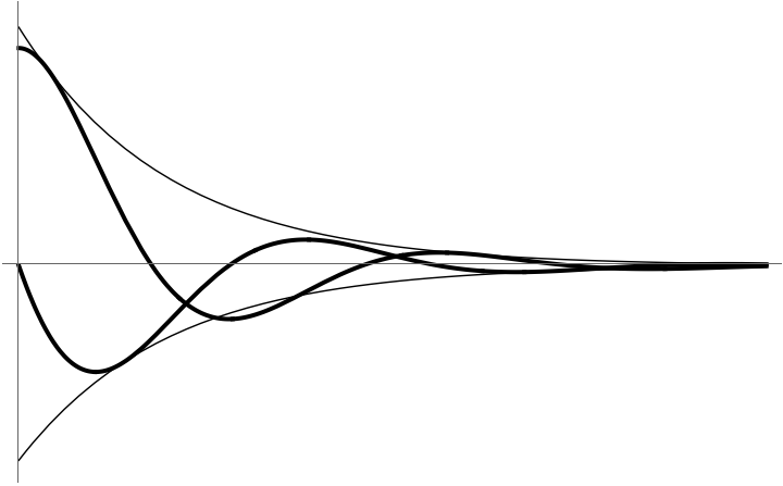
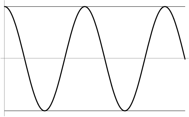
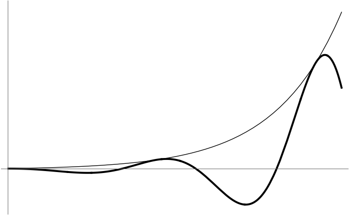
- Both Equation 4 and Equation 5 are equivalent ways of referring to the same phenomenon:
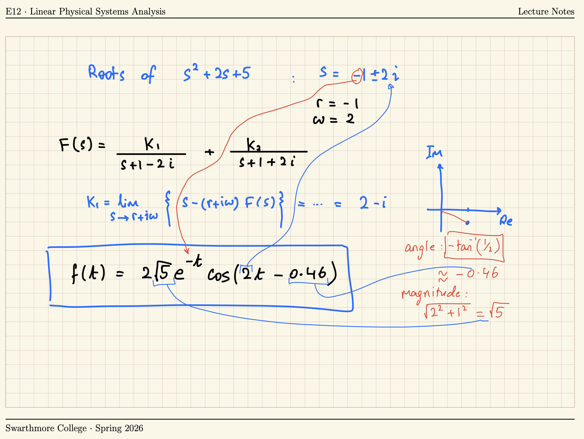
Practice
Find the inverse Laplace Transform of the following function: \[F(s) = \frac{4s+8}{s^2+2s+5}\]
Forced Response of 2nd order systems
| Input | \(f(t)\) | \(F(s)\) | Response \(X(s)\) | Response \(x(t)\) |
|---|---|---|---|---|
| Step |
\(b u_s(t)\) | \(\displaystyle \frac{b}{s}\) | \(\displaystyle \frac{b}{s} \frac{\omega_n^2}{s^2 + 2 \zeta \omega_n s + \omega_n^2}\) | \(\displaystyle \phantom{\frac{b}{a} \left( 1 - e^{-at} \right)}\) 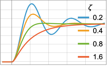 |
| Impulse |
\(A \delta(t)\) | \(A\) | \(A \displaystyle \frac{\omega_n^2}{s^2 + 2 \zeta \omega_n s + \omega_n^2}\) | \(\displaystyle \phantom{A e^{-at}}\) 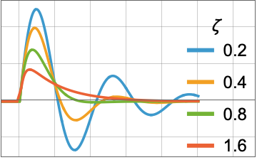 |
| Ramp |
\(u_s(t) \cdot c t\) | \(\displaystyle \frac{c}{s^2}\) | \(\displaystyle \left(\frac{c}{s^2}\right) \frac{\omega_n^2}{s^2 + 2 \zeta \omega_n s + \omega_n^2}\) | \(\displaystyle \phantom{\frac{c}{a^2} \left( e^{-at} - 1\right) + \frac{c}{a} t}\) 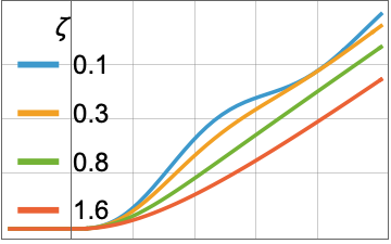 |
| Sinusoid |
\(u_s(t) \cdot \sin \omega t\) | \(\displaystyle \frac{\omega}{s^2+\omega^2}\) | \(\displaystyle \left(\frac{\omega}{s^2+\omega^2} \right) \frac{\omega_n^2}{s^2 + 2 \zeta \omega_n s + \omega_n^2}\) | 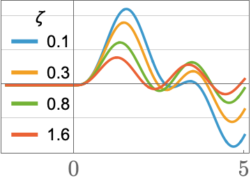 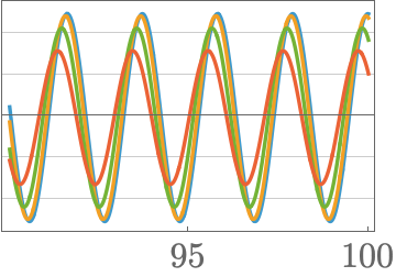 |