Lecture 2

E12 Linear Physical Systems Analysis

Prof. Emad Masroor

2026-01-22

Announcements

• HW 0 is due tonight
• HW 1 will be released tonight, due next Thursday
• New: Wizards will hold weekly individual office hours in Singer 228 on Mon, Tue, Wed and Thu.
• New: Lecture reflection: an anonymous ‘digital notecard’ system for collecting short-form feedback. Any responses will be addressed in the very next lecture if possible.
  • Have a question about lecture and don’t have time to ask in person right afterward? Fill out the form!
  • Other uses: notice a mistake, ask for a missing step in a derivation, point of clarification, etc.
• Minitutorial on matrices and vectors
  • What? matrix-vector equations, dot products, matrix inverse, etc.
  • When/Where? Monday, Jan 26 6:15 PM during Problem Session at Singer 222

Linearizing a nonlinear system

The input of a certain system is \(x\) and the output is \(f(x)\), and the inputs and outputs are related as

\[f(x) = x^2 - 3 x + 1\]

Quickly plotting functions

You should be familiar with at least one technique for quickly plotting a function using a calculator or computer. I like Mathematica for this purpose. You are recommended to use a program that can easily export plots as images.

• We are looking for a linear approximation to \(f(x)\), i.e., \(f^*(x) \approx f(x)\) where \(f^*(x)\) is linear in \(x\).

• Task 1: Write down a linear model \(f^*(x)\) for this system that is applicable everywhere

  • This is not possible

• Task 2: Write down a linear model \(f^*(x)\) for this system that is applicable:

  • near \(x=0\)
  • near \(x=3\)

We can linearize nonlinear systems for a while

Math in E12

Review from before

• Complex arithmetic
• Vectors
  • Also matrices; come to Monday’s minitutorial if needed
• Integration & Differentiation
• Partial fractions
  • We will extensively use, but also review.

New in E12

• Linear Constant-coefficient 2nd order differential equations
• Laplace transforms
• Manipulating matrices and vectors
• The Dirac delta function and the Heaviside Step function
• Fourier Series representation of arbitrary periodic functions.

Complex numbers

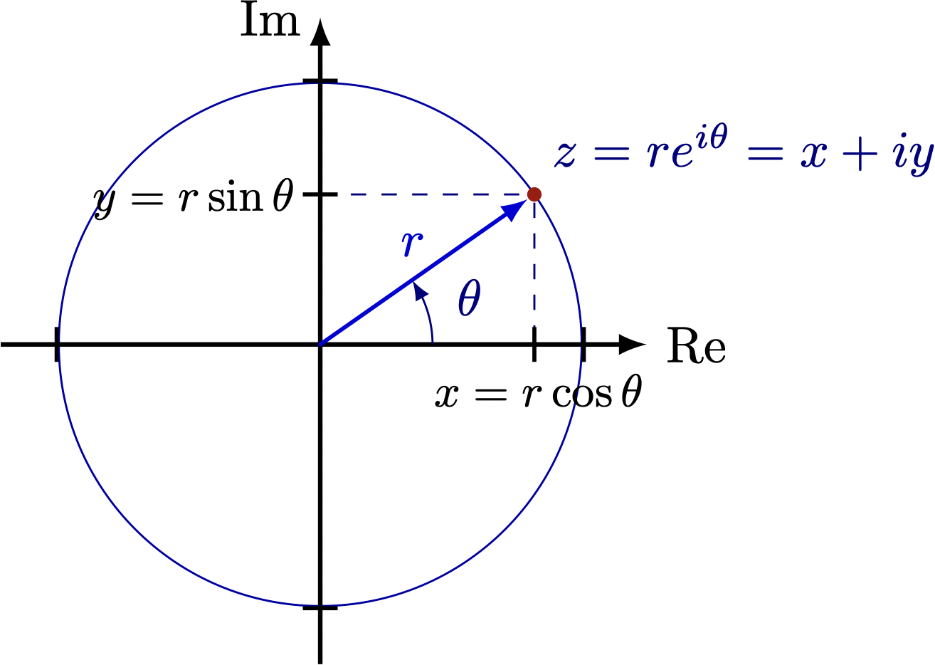
• A complex number \(z\) is the sum of a real part and an imaginary part \[z = x + i y\]
• where \(i\) is the imaginary unit \[i^2 \equiv -1 \]
• Complex numbers can be written in Cartesian or polar form. Magnitude of \(z\) is \(r\) and Argument of \(z\) is \(\theta\).

Arithmetic on Complex numbers

\[\text{ Let } z_1 = x_1 + i y_1, \quad z_2 = x_2 + i y_2\]

• Complex numbers can be added by separately adding their real and imaginary parts \[z_1 + z_2 = (x_1 + x_2) + i (y_1 + y_2)\]

• Complex numbers can be multiplied by distributing out the terms in Cartesian form: \[z_1 z_2 = (x_1 + i y_1)(x_2 + i y_2) = x_1 x_2 + i x_2 y_1 + i x_1 y_2 + i^2 y_1 y_2\]

• or by using their polar form and multiplication laws for exponentials \[z_1 z_2 = r_1 r_2 e^{i(\theta_1+\theta_2)}\]

• the ‘Complex Conjugate’ \(\bar{z}\) of a complex number \(z = x+ i y\) is defined as \[\bar{z} \equiv x - i y\]

Practice with Complex Numbers

For these tasks, remember that any complex number \(z = x+ i y\) can be thought of as a vector pointing from the origin to \([x,y]\).

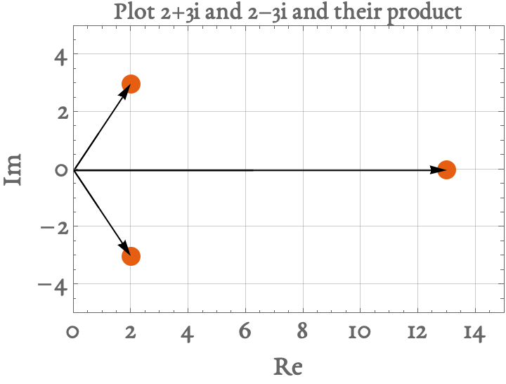
1. Plot \(2+3i\) and its complex conjugate in the complex plane. Multiply these two numbers and interpret the result geometrically
2. Calculate \(2 + 3i\) divided by \(3-7i\) and express the answer with no \(i\) in the denominator
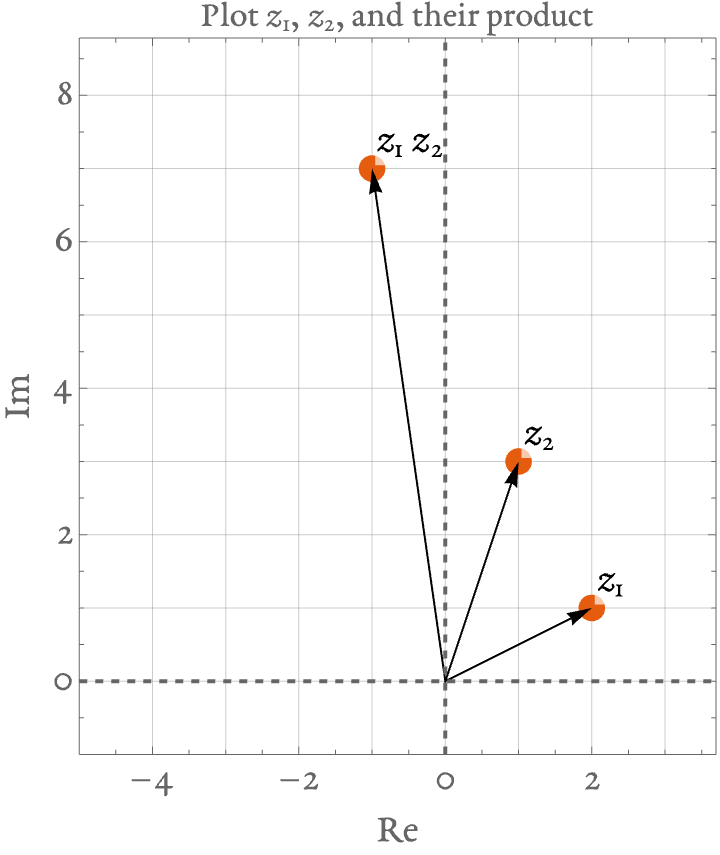
3. Choose any two complex numbers \(z_1\) and \(z_2\) and plot on the complex plane. What does \(z_1 z_2\) represent geometrically
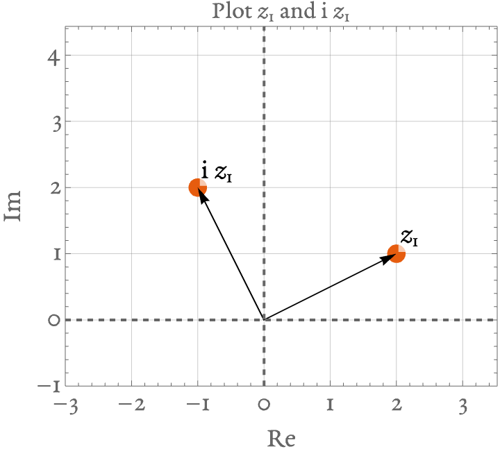
4. Geometrically, what does multiplying by an imaginary number (start with \(1i\)) do to a number on the complex plane?
5. Geometrically, what does multiplying by a real number do to a number on the complex plane?
6. Derive Euler’s identity \[e^{i \pi} + 1 = 0\]

Answers below

1. The result is a real number equal to \(2^2+3^2\).

2. \[\frac{2+3i}{3-7i} = \frac{2+3i}{3-7i} \frac{3+7i}{3+7i} = \frac{27-5i}{9+49} = \frac{27}{58} - i \frac{5}{58} \]

3. Their arguments get added to each other and their magnitudes get multiplied to each other.

4. It rotates the number by 90 degrees.

5. It stretches the number by a factor.

6. To ‘prove’ (not in the mathematical sense) Euler’s identity, we have to notice that \(e^{i\pi} = -1.\) Why would this be the case? The answer is that, on the unit circle in the complex plane, the number \(z=-1+0i\) is located on the negative real axis and has ‘angle’ 180 degrees.

Physical Systems that change with time

Using the convention that the overdot represents a time-rate of change, we can write a first-order differential equation for a system that changes with time: \[\frac{d\boldsymbol{x}}{dt} \equiv \dot{\boldsymbol{x}} = f(\boldsymbol{x},t)\]

• \(\boldsymbol{x}\): What system is like right now. Scalar or vector.

• \(\dot{\boldsymbol{x}}\): Rate of change of \(x\) with respect to time.

• An alternative approach:

What kinds of physical systems?

• In this class, we are primarily interested in first- and second- order systems. \[ \begin{aligned} \frac{d\boldsymbol{x}}{dt} \equiv \dot{\boldsymbol{x}} &= f(\boldsymbol{x},t) \\ \frac{d^2\boldsymbol{x}}{dt^2} \equiv \ddot{\boldsymbol{x}} &= f(\boldsymbol{x},\dot{\boldsymbol{x}},t) \end{aligned} \]

• Additionally, in our class:

  • \(f\) will be linear in \(x\) and \(\dot{x}\), but not necessarily in \(t\)
  • \(f\) will (possibly) be a function of time but \(f\) does not change with time

• Equations are linear in \(\boldsymbol{x}\) → Can be written in matrix-vector form.

\[ \begin{aligned} \frac{d}{dt} \begin{bmatrix} x_1 \\ x_2 \end{bmatrix} &= \begin{bmatrix} a & b \\ c & d \end{bmatrix} \begin{bmatrix} x_1 \\ x_2 \end{bmatrix} \\ \frac{d \boldsymbol{x}}{dt} &= \boldsymbol{A} \boldsymbol{x} \end{aligned} \]

Classification of Physical Systems

From Close, Frederick and Newell Chapter 1.4:

Criterion	Classification
Spatial characteristics	Lumped parameters
	Distributed parameters
Continuity of time variable	Continuous
	Discrete
Parameter variation	Fixed
	Time-varying
Superposition property	Linear
	Nonlinear

E12 is concerned with continous, time-invariant, linear, lumped-parameter systems

What does ‘lumped parameters’ mean?

• Lumped parameters assumption allows us to use ordinary differential equations instead of partial differential equations to model the system.

The order of a differential equation

The order of a differential equation is the highest derivative that appears in it.

• All first-order differential equations can be written in the following form: \[\dot{x} = f(t,x) \tag{1}\]

• All second-order differential equations can be written in the following form: \[\ddot{x} = f(t,x,\dot{x}) \tag{2}\]

• An \(n^{\text{th}}\) order differential equation can be written in the form \[\frac{d^n x}{dt^n} = f(t,x,\dot{x}, \ddot{x}, \dddot{x}, x^{(4)}, ..., x^{(n-1)} ) \tag{3}\] where \(x^{(n)}\) is shorthand for \({d^n x}/{dt^n}\)

• Later, we will learn that all \(n^{\text{th}}\) order differential equations can be re-arranged as a set of \(n\) first-order equations.

Coupled vs. uncoupled differential equations

• The following set of equations is uncoupled because the two equations are not ‘tied together’ in any way. \[ \begin{aligned} \dot{x} &= 2x + t \\ \dot{y} &= 3y + t \end{aligned} \]

• The following set of equations is coupled because the two equations are ‘tied together’. \[ \begin{aligned} \dot{x} &= 2x + t \\ \dot{y} &= 3x + t \end{aligned} \]

• Coupling can be one way (A depends on B but B does not depend on A) \[ \begin{aligned} \dot{x} &= 2x \\ \dot{y} &= 3x \end{aligned} \]

• or two-way (A depends on B and B depends on A) \[ \begin{aligned} \dot{x} &= 2y \\ \dot{y} &= 3x \end{aligned} \]

‘Element Laws’

• In analyzing physical systems, we would like to ‘break up’ a complicated physical system into its constituent parts.

• For each part, we can write an ‘element law’, i.e., a law of physics that we assume the part (or ‘element’) will obey.

Element laws for (translational) mechanical systems

Mass

• \(\displaystyle M \frac{d v}{dt} = f\)

Element laws for (translational) mechanical systems

Friction

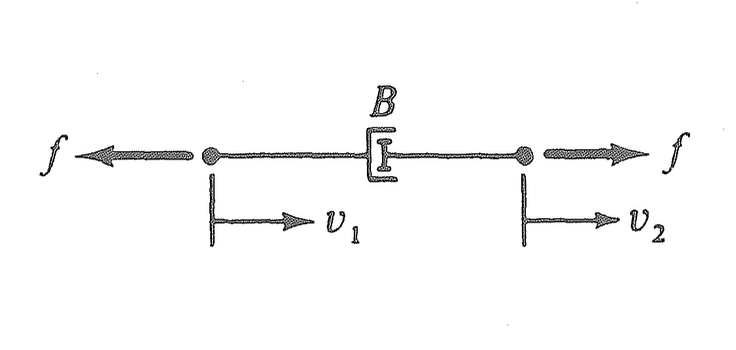
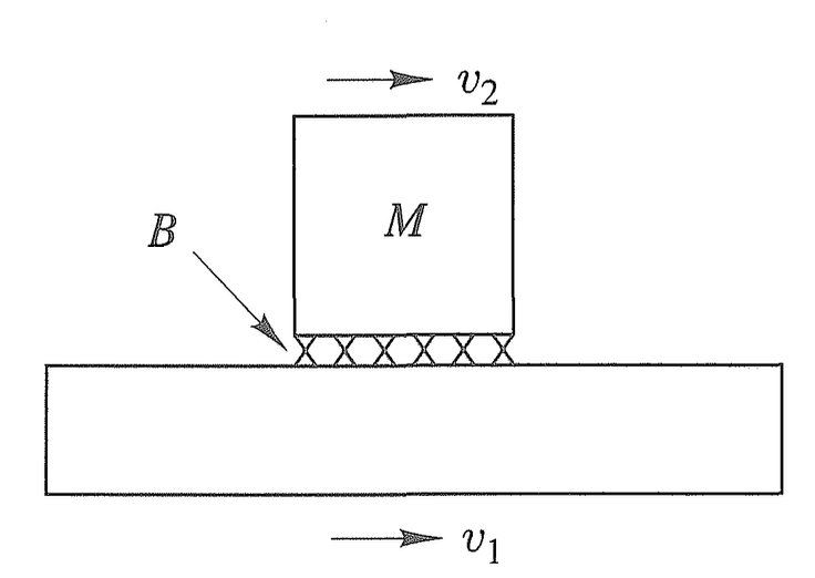
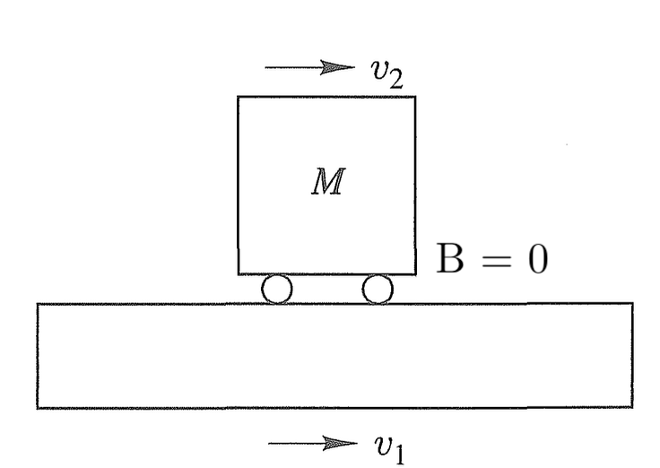
• \(\displaystyle B (v_2-v_1) = f\)
• in practice, we make models in which \(v_1\) or \(v_2 = 0\)
• force always opposes motion

Element laws for (translational) mechanical systems

Stiffness i.e. Springs

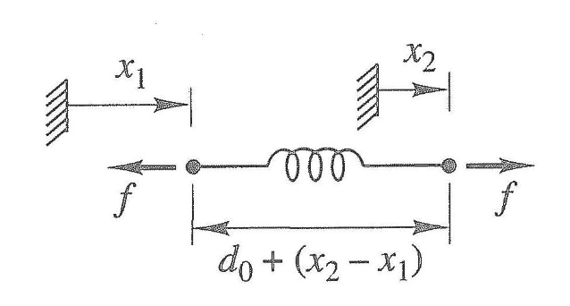
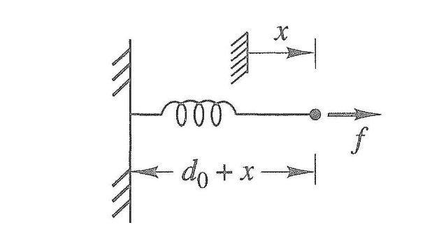
• \(\displaystyle K (x_2-x_1)) = f\) a.k.a Hooke’s Law

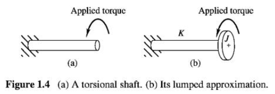
Element laws for rotational mechanical systems

Rotational analog for mass

• Instead of Mass, we have Moment of Inertia \[M\frac{dv}{dt} = F \quad \rightarrow \quad J \frac{d \omega}{dt} = T\]

• \(T\) is ‘torque’

• \(\omega\) is the angular velocity in radians per second

• \(J \omega\) is the angular momentum

• \(J\) is the ‘Mass moment of inertia’ \(\displaystyle \int r^2 dm\)

  • Formulas are available for many shapes’ moments of inertia

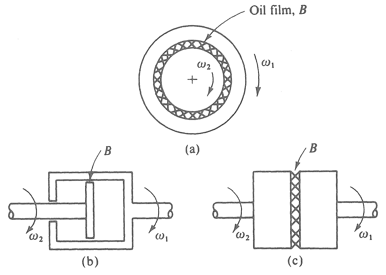
Element laws for rotational mechanical systems

Rotational analog for friction

\[M\Delta v = F \quad \rightarrow \quad B \Delta \omega = T\]

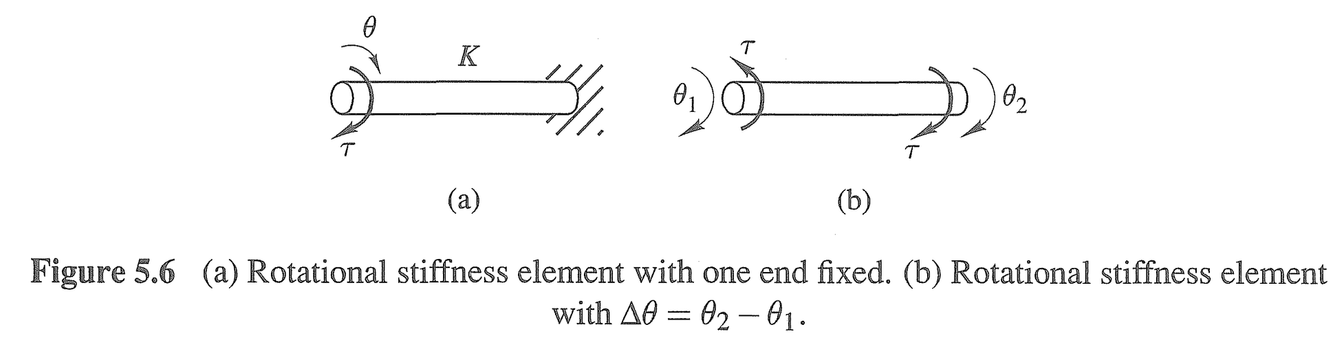
Element laws for rotational mechanical systems

Rotational analog for stiffness i.e. rotational springs

\[K (x_2-x_1)) = F \quad \rightarrow \quad K \Delta \theta = T\]

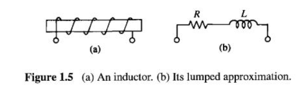
Element laws for electrical systems

Resistor

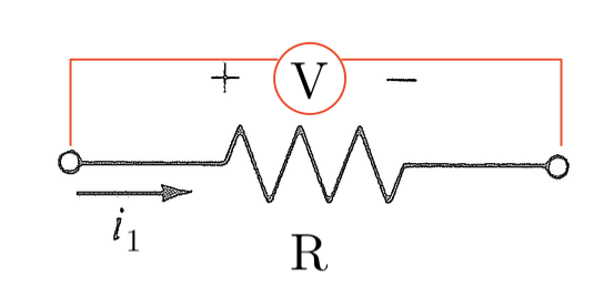
\(\displaystyle i_1 = \frac{1}{R} V\)

Capacitor

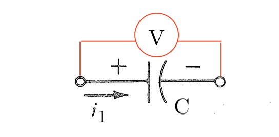
\(\displaystyle i_1 = C \frac{dV}{dt}\)

Inductor

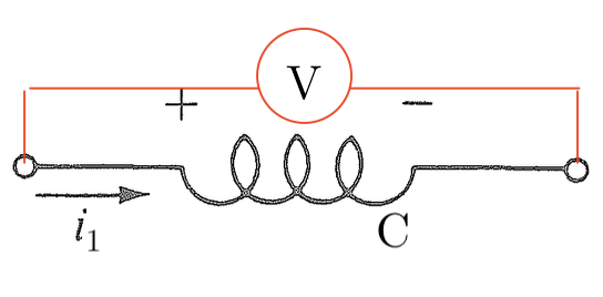
\(\displaystyle V = L \frac{d i_1}{dt}\)

Analyzing a linear physical system

Mechanical

\[M \frac{dv}{dt} + b v = 0\]

Electrical

Figure 1: An RC Circuit. \(V\) refers to the voltage across either the resistor or the capacitor; they’re the same.

\[\frac{dV}{dt} + \frac{1}{RC}V = 0\]

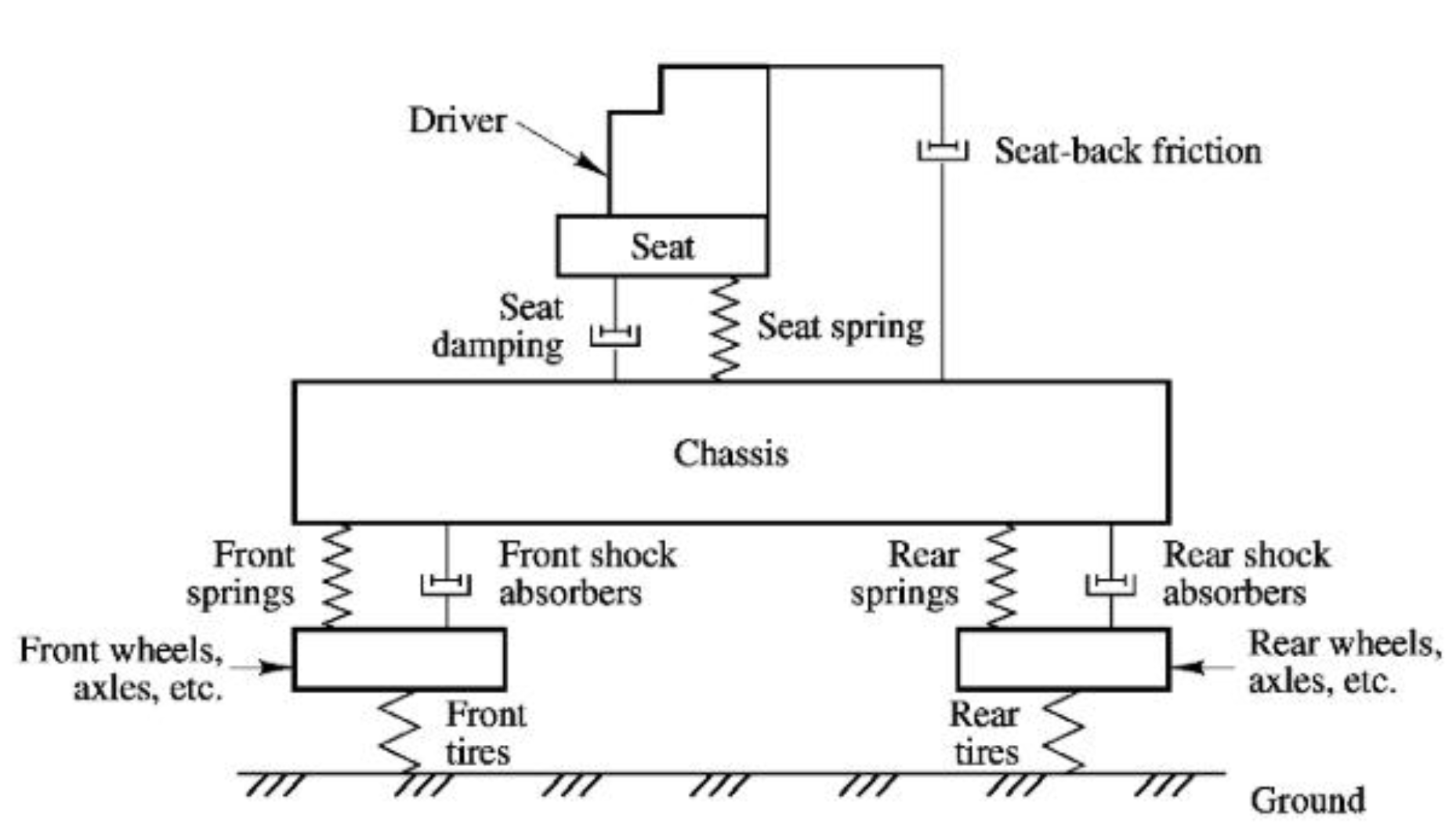
A coupled linear physical system

Let’s develop (not solve yet!) the equations for such a system.