Lecture 23
E12 Linear Physical Systems Analysis
April 14, 2026
Multiple-Input, Multiple-Output systems
There are multiple options for how to write down the equations of a system. Let’s look at two.
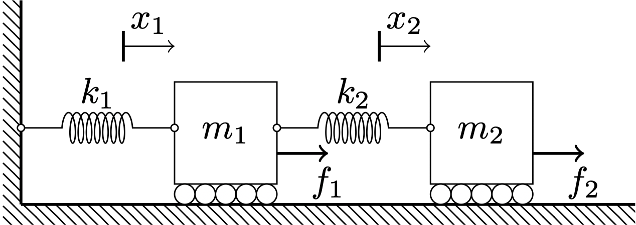
- Four state variables: \(x_1\), \(\dot{x}_1\), \(x_2\), \(\dot{x}_2\).
- Two inputs: \(f_1(t)\) and \(f_2(t)\).
- We are interested in three outputs:
- The position of the first mass \(x_1\)
- The distance between the two masses, \(x_2-x_1\)
- The total momentum of the system, \(m_1 \dot{x}_1 + m_2 \dot{x}_2\)
- Four state variables: \(x_1\), \(\dot{x}_1\), \(x_2-x_1\), \(\dot{x}_2\).
- Two inputs: \(f_1(t)\) and \(f_2(t)\).
- We are interested in three outputs:
- The position of the first mass \(x_1\)
- The position of the second mass, \(x_2\)
- The total potential elastic energy of the system, \(\frac{1}{2}k {x_1}^2 + \frac{1}{2} k x_2^2\)
Constructing the input control matrix
\[ \frac{d}{dt} \begin{bmatrix} x_1 \\ \dot{x}_1 \\ x_2 \\ \dot{x}_2 \end{bmatrix} = \begin{bmatrix} 0 & 1 & 0 & 0 \\ -(k_1+k_2)/m_1 & 0 & k_2/m_1 & 0 \\ 0 & 0 & 0 & 1 \\ k_2/m_2 & 0 & -k_2/m_2 & 0 \end{bmatrix} \begin{bmatrix} x_1 \\ \dot{x}_1 \\ x_2 \\ \dot{x}_2 \end{bmatrix} + {\color{red}{\begin{bmatrix} 0 \\ f_1/m_1 \\ 0 \\ f_2/m_2 \end{bmatrix}}} \]
We can re-write the equations of this system in the form \[\dot{\boldsymbol{x}} = \boldsymbol{A} \boldsymbol{x} + \boldsymbol{B} \boldsymbol{u}\]
where \(\boldsymbol{u}\) is a vector of inputs. Here, \(\boldsymbol{u} = \begin{bmatrix} f_1 \\ f_2 \end{bmatrix}\)
to find \(\boldsymbol{B}\) we construct a matrix of size \(n \times m\)
- here, \(n\) is the number of state variables and \(m\) the number of inputs.
\[ \underbrace{{\color{magenta}{\begin{bmatrix} 0 & 0 \\ 1/m_1 & 0 \\ 0 & 0 \\ 0 & 1/m_2 \end{bmatrix}}}}_{\boldsymbol{\displaystyle B}} \begin{bmatrix} f_1 \\ f_2 \end{bmatrix} = {\color{red}{\begin{bmatrix} 0 \\ f_1/m_1 \\ 0 \\ f_2/m_2 \end{bmatrix}}} \]
Constructing the (linear) output equations
We are interested in three specific outputs:
- The position of the first mass \(x_1\)
- The distance between the two masses, \(x_2-x_1\)
- The total momentum of the system, \(m_1 \dot{x}_1 + m_2 \dot{x}_2\)
- To construct the output equation \[{\boldsymbol{y}} = \boldsymbol{C} \boldsymbol{x} + \boldsymbol{D} \boldsymbol{u}\]
- we need to express the output variables of interest (\(\boldsymbol{y}\)) as a linear combination of
- the state variables (\(\boldsymbol{x}\)) and
- the input variables (\(\boldsymbol{u}\)).
- Let \(y_1 = x_1\)
- Let \(y_2 = x_2-x_1\)
- and \(y_3 = m_1 \dot{x}_1 + m_2 \dot{x}_2\)
- So we have \[\boldsymbol{C} = \begin{bmatrix} +1 & 0 & 0 & 0 \\ -1 & 0 & +1 & 0 \\ 0 & m_1 & 0 & m_2 \end{bmatrix}, \]
- multiplying \[ \boldsymbol{x} = \begin{bmatrix} x_1 \\ \dot{x}_1 \\ \dot{x}_2 \\ \dot{x}_2 \end{bmatrix} \]
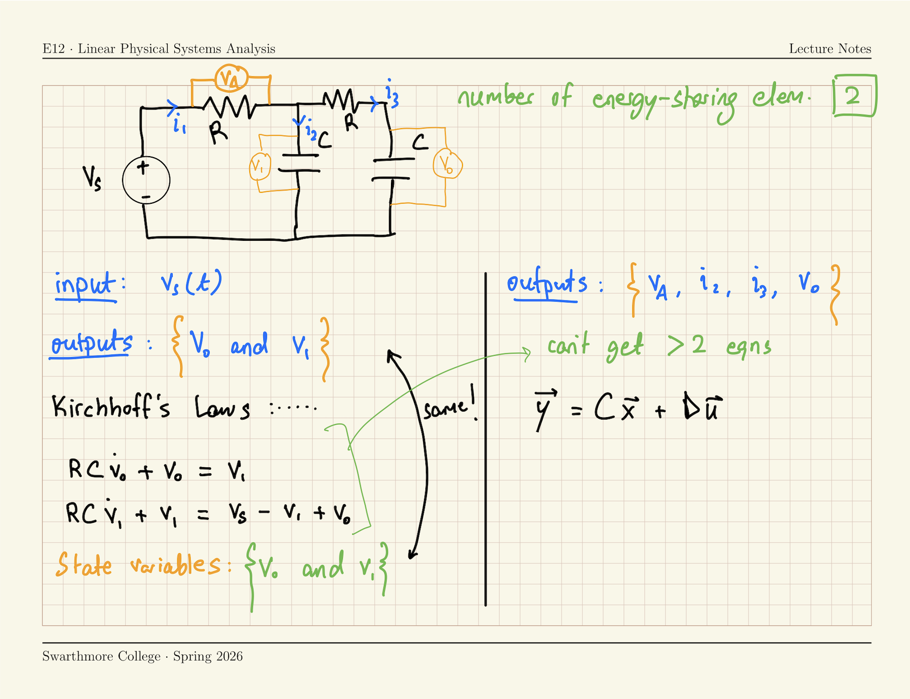
Two outputs in a circuit