Lecture 6
E12 Linear Physical Systems Analysis
February 5, 2026
Functions shifted in time: step function
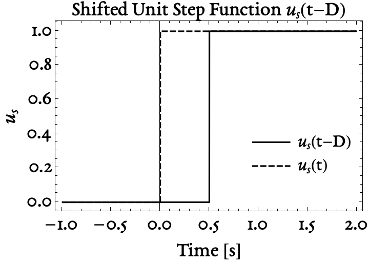
A step function applied with a delay of 0.5 seconds
Functions shifted in time: impulse function
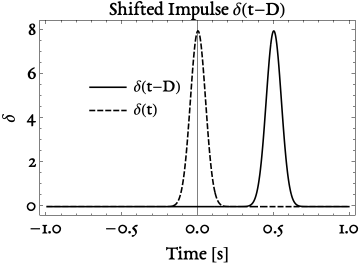
An impulse function applied with a delay of 0.5 seconds
Functions shifted in time: ramp function
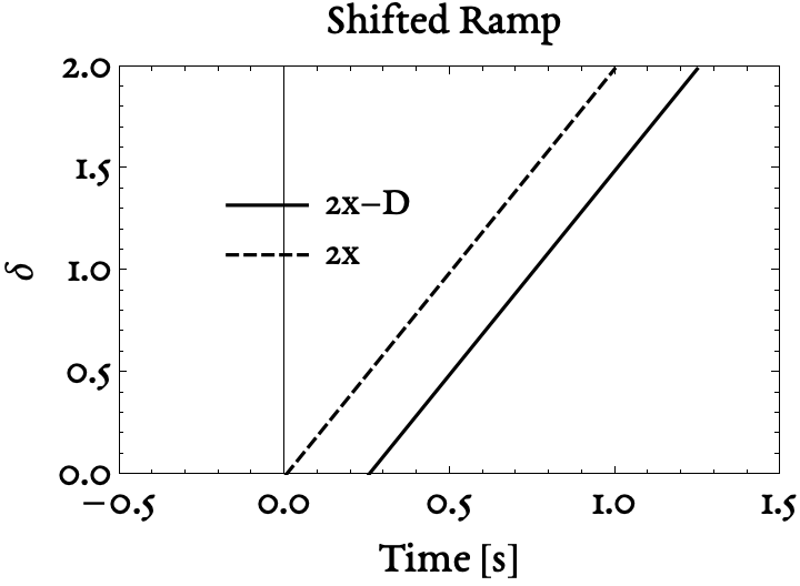
A ramp function applied with a delay of 0.5 seconds
Laplace Transform of a time-shifted function
If \[ f(t) = \begin{cases} 0 & t < D \\ g(t-D) & t > D \end{cases} \]
- Then the Laplace Transform of \(f(t)\) is \[\mathcal{L}[f(t)] = F(s) = e^{-sD} \mathcal{L}[g(t)] = e^{-sD} G(s)\]
Linear relation between input and output
in the frequency domain
\[\dot{x} + a x = f(t)\]
- Apply Laplace Transform \[\mathcal{L}[\dot{x}] + \mathcal{L}[a x] = \mathcal{L}[f(t)]\]
- Differential equation becomes algebraic equation \[sX(s) - x(0) + aX(s) = F(s)\]
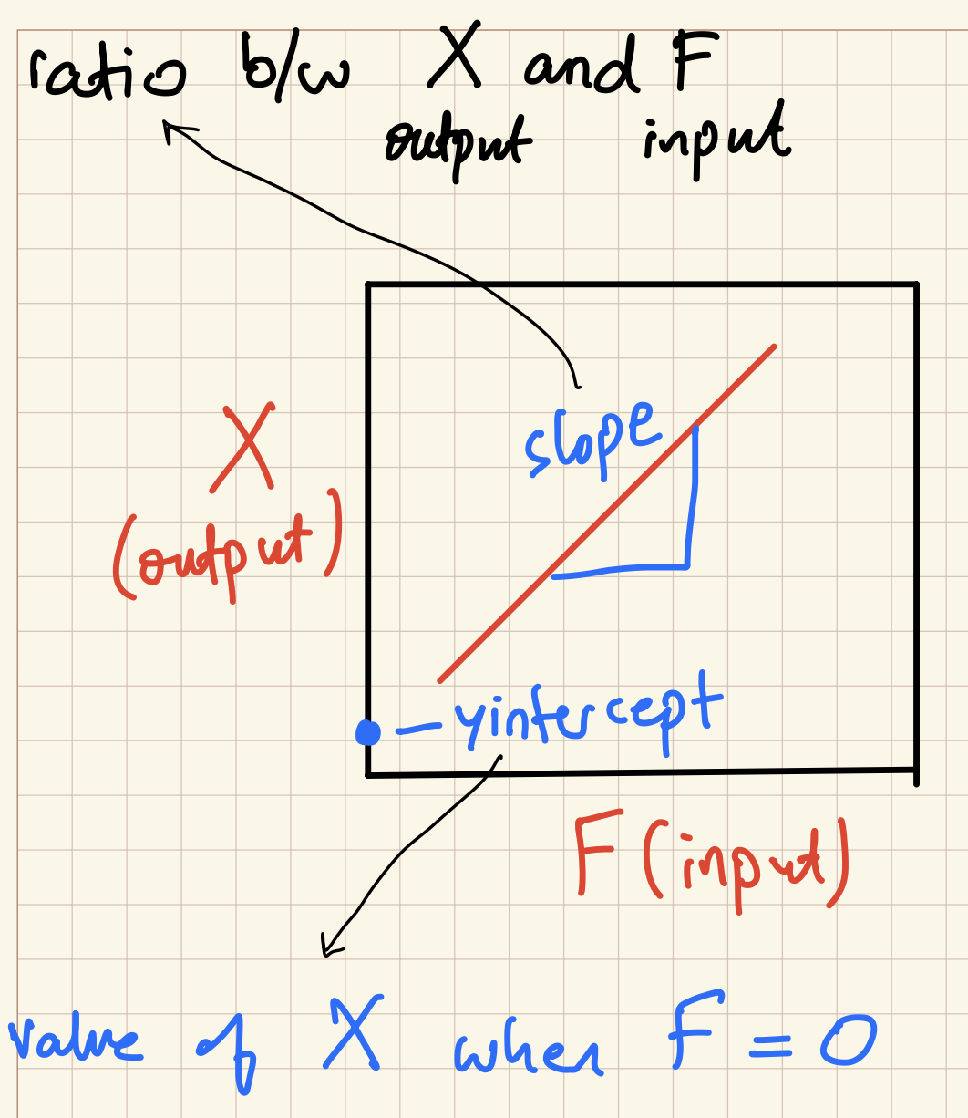
- Bringing (unknown) output to the left \[X(s) = \frac{F(s)}{s+a} + \frac{x(0)}{s+a}\]
- In-class task: Sketch graph of \(X\) against \(F\)
- …
- Resembles \(Y = m X + Y_{X=0}\)
Determining the Transfer Function for a system
In-class task Calculate the transfer function for the following system in terms of \(m\) and \(b\) (without values).
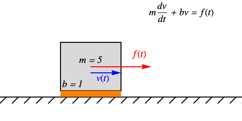
\[ \begin{aligned} m \dot{v} + b v = f(t) \implies m s V(s) + b V(s) &= F(s) \\ \implies V(s) \cdot (ms+b) = F(s) \implies \frac{V(s)}{F(s)} &= \frac{1}{ms+b} \end{aligned} \]
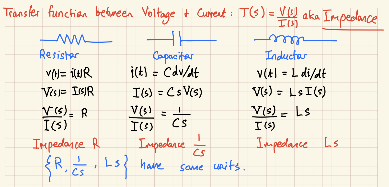
Transfer Functions for electrical components
In-class task If the voltage across the component is the output and the current through the component is the input, what is the Transfer Function for the following components? \[T(s) = \frac{V(s)}{I(s)}\]


Impedance and Transfer Functions
Calculating the free and forced response
The RC circuit shown here has governing equation \[RC \dot{v} + v = v_s, \quad v(0) = v_0\]

- In-class task Determine mathematical expressions for both the free and forced responses in frequency domain.
- Integrating in the time domain, we find \(v(t) =e^{-t/RC} \left( v_0 - v_s\right) + v_s\)
Using the Laplace Transform, we find \[ \begin{aligned} RC s V(s) - RC v(0) + V(s) &= \frac{v_s}{s} \\ RC s V(s) + V(s) &= \frac{v_s}{s} + RC v(0) \\ (RC s +1 )V(s) &= \frac{v_s}{s} + RC v_0 \\ V(s) &= \underbrace{\frac{v_s}{s} \times \overbrace{\frac{1}{RC s + 1}}^{\text{Transfer Function}}}_{\text{Forced Response}} + \underbrace{\frac{RC v_0}{RC s + 1}}_{\text{Free Response}} \end{aligned} \]
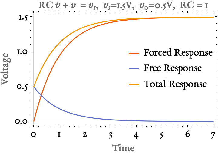
The forced response is \(v_s \left( 1-e^{-t/RC}\right)\) and the free response is \(v_0 e^{-t/RC}\)
Illustrating the forced and free response of an RC circuit to a constant input
\[v(t) = \left(v_s - v_s e^{-t/RC} \right) + \left( v_0 e^{-t/RC} \right)\]
Response of a 1st-order system to periodic input (system 1)
Response of a 1st-order system to periodic input (system 2)
Response of a 1st-order system to periodic input (system 3)
Effect of system parameters on response