ENGR 21 Fall 2025
HW 9
Summary
Due Date: Tue, Nov 11 at midnight
What to submit:
- A single PDF file Where to submit:
- PDF at this link
(1) Golden Section Search
(1.1) By hand
Use the Golden Section Search Method to locate the maximum of the function \(f(x) = -x^6 - 2 x^4 - 3 x^1 + 1\) between $x=-1$ and $x=0.5$. There is only one such maximum. Do this by filling out the following table up to the number of rows indicated, either by hand or electronically by downloading the $\LaTeX$ template.
(1.2) Pseudo-code
If you were to write a program that accomplishes what you did by hand in the previous part, what would you tell the program to do? Now that you are familiar with writing code for numerical methods in Python, write down the steps that you would ask the computer to take if you started with a bracket within which you know that a single root exists. Write your “program” in the form of a function that takes as input
- the function to be maximized, $f(x)$;
- the left and right edges of the bracket within which you know a maximum occurs. Call these $a$ and $b$.
- the required size of the final interval within which the solution should be bracketed, $\varepsilon$.
The output of your function should be the $x$-value of the midpoint of the final interval. This is your estimate of the maximum of $f(x)$.
Note
Pseudo-code can range from syntactically correct Python to plain English; don’t worry about exactly how to write it, as long as you get the general idea across. The common element is that pseudo-code should have the same structure as actual code, by indicating ‘for’ and ‘while’ loops as well as ‘if statements’, and should be appropriately indented to indicate the code that takes place under a certain loop or inside a certain ‘if’ or ‘else’ block.
(2) Naive multi-dimensional optimization
(2.1) Working out the steps by hand
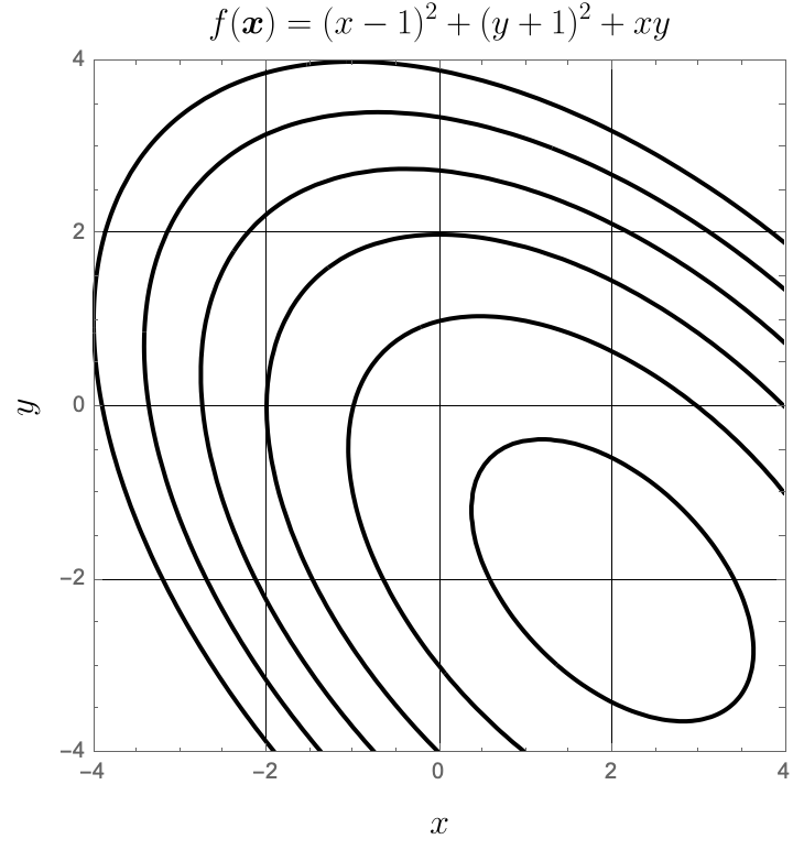
Minimize the function \(f(\boldsymbol{x}) = f(x,y) = (x-1)^2 + (y+1)^2 + xy \label{fmin}\) using naive $n$-dimensional optimization by hand for four steps, cycling through the direction vectors \(\boldsymbol{v_1} = \begin{bmatrix} 1 \\ 1\end{bmatrix}, \quad \boldsymbol{v_2} = \begin{bmatrix} 0 \\ 1 \end{bmatrix},\) starting with the guess \(\boldsymbol{x_0} = \begin{bmatrix} x_0 \\ y_0 \end{bmatrix} = \begin{bmatrix} -1 \\ 2 \end{bmatrix}.\) This function is simple enough that you should not need to use an optimization program to carry out each of the 1-dimensional optimizations; instead, you should be able to do these by hand using single-variable calculus.
At each step, calculate the ‘true relative error’ in $\boldsymbol{x}$ by comparing against the correct value of the minimum, and the `approximate relative error’ by comparing against the previously-computed value (i.e., compare step 1 against step 0, step 2 against step 1, etc.). These errors can be calculated using the following definitions:
\[\text{True relative error } = \frac{\left \lVert \boldsymbol{x} - \boldsymbol{x}_{\text{true}} \right \rVert }{ \left \lVert \boldsymbol{x}_{\text{true}} \right\rVert} , \text{ and}\] \[\text{Approximate relative error } = \frac{ \left\lVert \boldsymbol{x}_{\text{current}} - \boldsymbol{x}_{\text{previous}} \right \rVert}{ \left \lVert \boldsymbol{x}_{\text{previous}} \right \rVert}.\]Note that you can find the correct answer by solving a math problem; take derivatives of $f$ with respect to $x$ and $y$, equate them to zero, and solve the resulting equations ‘by hand’.
Also, recall that the norm of a vector is $\left \lVert \boldsymbol{x} \right \rVert = \sqrt{x_1^2+x_2^2 + … + x_n^2}$
Tabulate your results in the follwing format (there is no need to use square-root symbols though):
| Step 0 | Step 1 | Step 2 | Step 3 | Step 4 | |
|---|---|---|---|---|---|
| ( x ) | (-1) | ||||
| ( y ) | (\phantom{-}2) | ||||
| ( f(x,y) ) | (11) | ||||
| True relative error | ( \frac{5}{\sqrt{8}} \approx 1.768 ) | ||||
| Approx. relative error | N/A |
(2.2) Illustrate
Illustrate
Illustrate the steps from the previous problem graphically on the following plot, which shows contours of $f(\boldsymbol{x})$. Label the points $\boldsymbol{x}_0$ through $\boldsymbol{x}_4$, as well as the direction vectors $\boldsymbol{v}_1$ and $\boldsymbol{v}_2$ drawn at the appropriate locations. Altogether, you will have five points connected by four lines: two lines will have the direction of $\boldsymbol{v}_1$ and two will have the direction of $\boldsymbol{v}_2$. You may either use repeated labels or label the successive directions $[\boldsymbol{v}_1, \boldsymbol{v}_2, \boldsymbol{v}_3, \boldsymbol{v}_4]$