ENGR 21 Fall 2025
Resources
- Resources
- External Guides and Tutorials
- Instructor’s Circuit Playground Guide for E21
- Links and Code Snippets
- Lec 1.1, Tue Sep 2
- Lec 2.1, Tue Sep 9
- Lec 2.2, Thu Sep 11
- Lec 3.1, Tue Sep 16
- Lec 3.2, Thu Sep 18
- Lec 4.1, Tue Sep 23
- Lec 4.2, Thu Sep 25
- Lec 5.1, Tue Sep 30
- Lec 5.2, Thu Oct 2
- Lec 6.1, Tue Oct 7
- Lec 6.2, Thu Oct 9
- Lec 8.2, Thu Oct 30
- Lec 9.2 Thu, Nov 4
- Lec 10.1 Tue, Nov 11
- Lec 10.2 Thu, Nov 13
- Lec 11.1, Tue, Nov 18
- Lec 11.2, Thu, Nov 20
External Guides and Tutorials
- Official Python website
- Virtual Environments in Python
- Official CircuitPython documentation — use this page to look up the full documentation for functions.
- Download Mu, the simple IDE for Python and CircuitPython
- Download CircuitPython for the Circuit Playground Bluefruit
- Product page for the Circuit Playground Bluefruit
- Official Guide for the Circuit Playground Bluefruit
If Mu does not work for you on Windows, you can follow these instructions to use PuTTY as your console as an alernative.
Instructor’s Circuit Playground Guide for E21
To use any of these features, make sure your Python code includes the following line at the top:
from adafruit_circuitplayground import cp
Taps and shakes
cp.shake()  # Returns True if it's currently being shaken
cp.shake(shake_threshold=20)  # optional parameter to change sensitivity

cp.tapped # Returns True if it's currently being tapped
cp.detect_taps  # A variable that can be set to either 1 or 2; 2 looks for double taps.
Switching on the Red LED
cp.red_led = True # switches on the red LED
Detecting state of Slide switch
cp.switch # returns True or False
Using the Neopixels
There are 10 neopixels. The state of each is determined by a 3-tuple of RGB values, i.e. (p,q,r) where each element of the tuple is an integer between 0 and 255 and represents the red, green and blue channels respectively.
The full state of the neopixels is determined by a 10-element list of 3-tuples, i.e., 30 numbers in total, arranged in the form
[(0, 0, 0), (0, 0, 0), (0, 0, 0), (0, 0, 0), (0, 0, 0), (0, 0, 0), (0, 0, 0), (0, 0, 0), (0, 0, 0), (0, 0, 0)]
the variable cp.pixels contains the above list.
You can set individual elements of the neopixels, e.g., turn the 4th pixel to a mild green like so:
cp.pixels[4] = (0,10,0) # for pixel number 4, set red to 0, green to 10, and blue to 0
There is also a convenient method, cp.pixels.fill(), which you can use to control all the pixels at the same time. You must pass a 3-tuple to this method.
cp.pixels.fill((10,0,0)) # set red channel to a strength of 10 for all the neopixels.
Reading the light sensor
The light sensor on the Circuit Playground Bluefruit detects ambient light and returns an integer between 0 and ?. Access the curent reading of the light sensor using
cp.light
Reading raw data from the accelerometer
Access the raw data from the accelerometer in meters per seconds squared using
cp.acceleration
This yields an object of class acceleration with three attributes: x, y, and z. Thus,
cp.acceleration.z
returns the acceleration in the z direction.
Physical buttons A and B
There are two buttons on the Circuit Playground Bluefruit, labeled A and B. The boolean variables
cp.button_a
cp.button_b
are True while the corresponding buttons are pressed.
Temperature sensor
The temperature sensor on the Circuit Playground Bluefruit detects ambient temperature and returns a real number equal to the temperature in Celsius. Access the current temperature in Celsius using
cp.temperature
Capacitive Touch
Seven of the pins on the Circuit Playground Bluefruit can take capacitive touch input. image
These are A1, A2, A3, A4, A5, A6, and TX. You can see these names on the capacative input regions on the edges of the board, i.e. the mounting holes. The variable cp.touch_A1 will be True when pin A1 is being touched, and will be False otherwise. Thus, there are seven such variables:
cp.touch_A1cp.touch_A2cp.touch_A3cp.touch_A4cp.touch_A5cp.touch_A6cp.touch_TX
Speaker
- Play a tone at a frequency of x Hz for a duration of y seconds using
cp.play_tone(x,y). - Start playing a tone at a frequency of x Hz using
cp.start_tone(x) - Stop playing the currently-playing tone using
cp.stop_tone() - Play a
*.wavfile usingcp.play_file("filename.wav"). The file should be stored on theCIRCUITPY` drive.
Links and Code Snippets
Lec 1.1, Tue Sep 2
Installation Instructions
- Installing Circuit Python on your Circuit Playground Bluefruit. This will install Circuit Python, a compact and pared-down version of Python for embedded systems.
- Installing Mu on your computer. This is the IDE that we will use for Circuit Playground.
- Downloading Libraries and copying them on to Circuit Playground Bluefruit. Make sure you use the libraries from Circuit Python 9! Note that you must copy 2 folders and 3 files into the
libfolder of your Circuit Playground device.
Sample First Code to run on your board
from adafruit_circuitplayground import cp

while True:
    cp.pixels[4] = (10,0,10)
    if cp.button_a:
         cp.play_tone(440,1)
    if cp.button_b:
         cp.play_tone(220,1)
Lec 2.1, Tue Sep 9
read_pinA1_as_digital_input.py
from adafruit_circuitplayground import cp
import time

for j in range(200):
    print("Pin A1 digital read:",cp.touch_A1)
    print((int(cp.touch_A1),))
    if cp.touch_A1:
        cp.pixels[3] = (0,25,0)
    else:
        cp.pixels[3] = (25,0,0)
    time.sleep(0.1)
read_pinA1_as_analog_input.py
import board
import analogio
import time

pin_a1 = analogio.AnalogIn(board.A1)

for j in range(200):
    print("Pin A1 analog read:",pin_a1.value)
    print((pin_a1.value,))
    time.sleep(0.1)
read_pinA1_as_analog_input_v2.py
import board
import analogio
import time
import neopixel

pin_a1 = analogio.AnalogIn(board.A1)
pixels = neopixel.NeoPixel(board.NEOPIXEL, 10, auto_write=False)

for j in range(200):
    print("Pin A1 analog read:",pin_a1.value)
    print((pin_a1.value,))
    mapped_brightness = 150 # change this!
    pixels[3] = (0,mapped_brightness,0)
    pixels.show()
    time.sleep(0.1)
Lec 2.2, Thu Sep 11
(0) Code for Truth Table
# Set the values of A and B
A = True
B = False

# Implement “Logic gate OR” by covering all four possibilities.

if A == True:
    if B == True:
        C = True # line 1 of table
    else:
        C = True # line 2 of table
else:
    if B == True:
        C = True # line 3 of table
    else:
        C = False # line 4 of table

print("--After applying logic, C is",C)
(1) Code for time package
from adafruit_circuitplayground import cp

import time

delay = 3.0

print("Switching on pixel 0")
cp.pixels[0] = (0,10,0)
print(f"Waiting for {delay} seconds")
time.sleep(delay)

print("Switching on pixel 1")
cp.pixels[1] = (10,0,0)
print(f"Waiting for {delay} seconds")
time.sleep(delay)

print("Switching on pixel 2")
cp.pixels[2] = (0,0,10)
print(f"Waiting for {delay} seconds")
time.sleep(delay)
(2) Code for print statements
print(“The number is 24”)

p = 24.1
n = 24

print(“The numbers are n and p”)

print(“The numbers are {n} and {p}”)

print(f“The numbers are {n} and {p}”)

print(f"The numbers are {n:} {p:.3f}")

c = "The numbers are {} and {}".format(p,n)
print(c)
(3) Code for for loops
# Iterable (1): Range
print("Printing fron a range:")
for j in range(2,10,2):
    print(j)

# Iterable (2): list
print("Printing fron a list:")
a = [1,"a",6,"hello",5,True]
for j in a:
    print(j)

# Iterable (3): tuple
print("Printing fron a tuple:")
b = (1,2,"x",3,1)
for k in b:
    print(k)

# Iterable (4): string
print("Printing characters from a string:")
c = "hello"
for x in c:
    print(x)
(4) The break keyword
# break inside for loop
for j in range(10):
    print(j)
    if j == 3:
        print("exiting loop")
        break

# break inside while loop
counter_variable = 0
while 3 > 2:
    counter_variable += 1
    if counter_variable > 3:
        break
(5) The continue keyword
# break inside for loop
for j in range(10):
    print(j)
    if j == 3:
        print("exiting loop")
        break

# break inside while loop
counter_variable = 0
while 3 > 2:
    counter_variable += 1
    if counter_variable > 3:
        break
(6) Light up neopixels
from adafruit_circuitplayground import cp
import time

cp.pixels[0] = (10,10,10)
time.sleep(1)
cp.pixels.fill((0,0,0))

cp.pixels[1] = (30,30,30)
time.sleep(1)
cp.pixels.fill((0,0,0))

cp.pixels[2] = (50,50,50)
time.sleep(1)
cp.pixels.fill((0,0,0))

cp.pixels[3] = (70,70,70)
time.sleep(1)
cp.pixels.fill((0,0,0))
Lec 3.1, Tue Sep 16
Accelerometer Code
from adafruit_circuitplayground import cp
import time

def std(data):
    mean = sum(data) / len(data)
    squared_diffs = [(x - mean) ** 2 for x in data]
    variance = sum(squared_diffs) / len(data)
    std_dev = variance ** 0.5
    return std_dev

def magnitude(a,b,c):
    return (a**2 + b**2 + c**2)**(1/2)

# Number of readings
N = 10

# Create a list that will store the readings
readings_z = [0] * N
readings = [0] * N

# Time delay between measurements
delay = 2

for j in range(N): # Number of seconds to run
    accel_z = cp.acceleration.z
    accel   = magnitude(cp.acceleration.x, cp.acceleration.y,cp.acceleration.z)
    print((accel_z,accel))
    readings[j] = accel
    readings_z[j] = accel_z
    time.sleep(delay) # delay of 1 second

avg_reading = sum(readings)/len(readings)
avg_reading_z = sum(readings_z)/len(readings_z)
print("After ",N," readings, the acceleration is ",avg_reading," m/s^2")
print("With standard deviation ",std(readings))
print("After ",N," readings, the z-acceleration is ",avg_reading_z," m/s^2")
print("With standard deviation ",std(readings_z))
Writing data to Circuit Playground Bluefruit
Copy the file boot.py into your CIRCUITPY drive. The contents of this file are shown below for reference.
"""CircuitPython Essentials Storage logging boot.py file adapted from Adafruit"""
import board
import digitalio
import storage

# For Circuit Playground Express, Circuit Playground Bluefruit
switch = digitalio.DigitalInOut(board.D7)

switch.direction = digitalio.Direction.INPUT
switch.pull = digitalio.Pull.UP

# If the switch pin is connected to ground CircuitPython can write to the drive
storage.remount("/", readonly=switch.value)
After you have saved this file to your CIRCUITPY drive, eject CIRCUITPY from your operating system, then press the rest button.
- If your slide switch is set toward the right (near button B) then your board can write files and your computer cannot write files to
CIRCUITPY. - If your slide switch is set toward the left (near button A) then your baord cannot write files and your computer can write files to
CIRCUITPY.
You can find an ‘official’ tutorial for how to use this file here.
Reaction times game
from adafruit_circuitplayground import cp
import time
import random

# Choose the number of data points to collect
N = 5

# Create a list to collect data points
data = [0] * N

# Print some information
print("Welcome to the reaction time game.")
print(f"We will collect {N} samples.")
print("Press button A when an LED lights up.")

# Open file for writing
f = open("/reaction_times.txt","a")
for j in range(N):
    # Turn off all LEDs
    cp.pixels.fill((0, 0, 0))

    # Wait for a random time between 1 and 5 seconds
    random_delay = random.uniform(1, 5)
    time.sleep(random_delay)

    # Turn on a random LED (pick an index from 0 to 9)
    led_index = random.randint(0, 9)
    cp.pixels[led_index] = (0, 10, 0)  # Green LED lights up

    # Record the time the LED lights up
    start_time = time.monotonic()

    # Wait for button A press
    while not cp.button_a:
        # do nothing; keep waiting in this while loop
        pass

    # Button pressed! First, calculate the reaction time.
    reaction_time = time.monotonic() - start_time

    # Switch off the LED
    cp.pixels[led_index] = (0, 0, 0)

    # Print the reaction time to the serial console
    print(f"Reaction time: {reaction_time:.3f} seconds")

    # Write to file
    f.write(f"{reaction_time:.4f}\n")
    f.flush()

    # Pause before restarting the game
    time.sleep(2)

# Close the file for writing.
f.close()
Lec 3.2, Thu Sep 18
Writing your own function
The following is some “starter code” for you to write your own function
from adafruit_circuitplayground import cp
import time
def lightUp(color,n,p):
    # Lights up pixel number n using color "color"
    # 'Color' should be a string, either 'red', 'blue', or 'green'
    # n should be an int between 0 and 9
    # p should be any number between 1 and 255
    return 42

# Now call it inside a while loop
while True:
    lightUp(‘red’,8,45)
    time.sleep(3)
    lightUp('green',5,200)
    time.sleep(3)
    cp.play_tone(440,3)
Lec 4.1, Tue Sep 23
Command Line Programs
import sys

name    = sys.argv[1]
num     = int(sys.argv[2])

print(f"This program prints {name} {num} times.")
for j in range(num):
    print(name)
Save the above code as script1.py. Then, run your code on the command line / terminal by entering:
python3 script1.py testname 5
Lec 4.2, Thu Sep 25
Floating-point IEEE Standard
Lec 5.1, Tue Sep 30
NumPy reference
See the official NumPy documentation here.
Floating Point Error Accumulation
import numpy as np

# Use NumPy's float16 type
a = np.float16(1e-3)  # A small number
n = 10000  # Large number of iterations

result = np.float16(0)  # Start with 0 in float16

# Add the small number 'a' to 'result' n times
for i in range(n):
    result += a

print("Expected result:", a * n)
print("Result with float16:", result)  # Result with float16
Breaking Floating point numbers
import numpy as np

def showFloat(number):
    # print(f"Binary representation of {number:.3f}, type {type(number)}:")
    if str(type(number)) == "<class 'numpy.float16'>":
        x = np.float16(number)
        bits = x.view(np.uint16)
        return f"{bits:016b}"
    elif str(type(number)) == "<class 'numpy.float32'>":
        x = np.float32(number)
        bits = x.view(np.uint32)
        return f"{bits:032b}"
    elif str(type(number)) == "<class 'numpy.float64'>":
        x = np.float64(number)
        bits = x.view(np.uint64)
        return f"{bits:064b}"
    else:
        print("Type is not compatible")

# Declare some 16-bit floating-point numbers
a = np.float16(128)
c = np.float16(16)
ep = np.float16(0.2)

# Add them together and print them out:

print('128 + 0.2 =',a+ep)
print('128 + 0.2 + 0.2 =',a+ep+ep)
print('128 + 0.2 + 0.2 + 0.2 =',a+ep+ep+ep)
print('128 + (0.2 + 0.2 + 0.2) =',a+(ep+ep+ep))
# View the internals
print(showFloat(a+(ep+ep+ep)))
print(showFloat(a+ep+ep+ep))
print('')

print('16 + 0.2 =',c+ep)
print('16 + 0.2 + 0.2 =',c+ep+ep)
print('16 + 0.2 + 0.2 + 0.2 =',c+ep+ep+ep)
print('16 + (0.2 + 0.2 + 0.2) =',c+(ep+ep+ep))

# View the internals
print(showFloat(c+(ep+ep+ep)))
print(showFloat(c+ep+ep+ep))
Lec 5.2, Thu Oct 2
Basic plotting syntax
import numpy as np
import matplotlib.pyplot as plt


xvals = np.linspace(0,2*np.pi,200)
yvals = np.sin(xvals)

plt.plot(xvals,yvals)
plt.show()
Different plotting styles
# Plot a sine curve
x = np.linspace(0,2*np.pi,20)
y = np.sin(x)

plt.plot(x,y,'o')
plt.show()


# Plot a sine curve
x = np.linspace(0,2*np.pi,15)
y = np.sin(x)

plt.plot(x,y,'o-')
plt.show()
Lec 6.1, Tue Oct 7
Bisection Algorithm
The following code almost implements the bisection algorithm. You must supply the code after the if-statements inside the while loop.
import math
from numpy import sign, cos, pi, exp, sin

def bisection(f,x1,x2,tol):
    # Carries out the bisection algorithm for the function f, using the
    # bracket (x1,x2) with a 'tolerance' of tol.
    f1 = f(x1)
    f2 = f(x2)
    if sign(f1) == sign(f2):
        # if the sign of f(x1) and f(x2) is the same,
        # there is probably no root between x1 and x2.
        print('Root is not bracketed between x1 and x2')
        return None

    er = 1 # some large value
    iters = 0
    while er > tol:
        iters+=1
        # uncomment the following line for debugging purposes
        # print(f'Root is between x1 = {x1:.3f} and x2 = {x2:.3f}')
        x3 = 0.5*(x1 + x2)
        f3 = f(x3)

        if f3 == 0.0:
            return x3
        if sign(f3) == sign(f2):
            # do something
            # new interval is ...
        else:
            # do something else
            # new interval is ...

        er = abs(x1-x2)
    return 0.5*(x1 + x2), iters

# Try it on the function 'cos'
bisection(cos,0.1,3.0,0.001)
Lec 6.2, Thu Oct 9
Lec 8.2, Thu Oct 30
Download the following files in zip format here.
| N | 6 | 60 | 200 |
|---|---|---|---|
| Matrix | matrix_A_6.csv | matrix_A_60.csv | matrix_A_200.csv |
| r.h.s | rhs_b_6.csv | rhs_b_60.csv | rhs_b_200.csv |
| solution | solution_x_6.csv | solution_x_60.csv | solution_x_200.csv |
Numpy’s built-in solver
import numpy as np

A = np.loadtxt('<filename>',delimiter=',')
b = np.loadtxt('<filename>',delimiter=',')

x = np.linalg.solve(A,b)
Conjugate Gradient Algorithm
import numpy as np
from numpy import transpose as tr
from numpy import dot

def conjugate_gradient(A,b,x_guess,tol=1e-6):
    # Uses the conjugate gradient method to solve Ax=b within tolerance specified by 'tol'.
    x = x_guess.copy()
    r = b - dot(A,x)
    beta = 0
    s = r.copy()

    while 2+2 == 4:
        a = dot(tr(s),r)/(dot(dot(tr(s),A),s))  # step size alpha
        x = x + a*s                             # update x
        r = b - dot(A,x)                     # calculate residual
        if norm(r) <  tol:
            break
        beta = - (dot(dot(tr(r),A),s)/
                  (dot(dot(tr(s),A),s)))        # step size beta
        s = r + beta*s                          # update search direction
    return x
Lec 9.2 Thu, Nov 4
Optimize the following function
def shearStress(y):
    return (61224.2 - 1.9334e6*y - 7.01705e8 * y**2 + 4.375e10 * y**3 - 6.81818e11 * y**4)/(0.000686111-0.053333*y+y**2)
Lec 10.1 Tue, Nov 11
1-dimensional optimization
from scipy.optimize import minimize_scalar
import numpy as np
from matplotlib import pyplot as plt

def test_f(x):
    return x**2 - 4*x + 7

solution = minimize_scalar(test_f,[-1,5])

print(f"Function minimized at x = {solution.x:.4f}")

x = np.linspace(-1,5)
plt.plot(x,test_f(x))
plt.grid()
plt.xlabel('y')
plt.ylabel('Shear stress')

plt.scatter(solution.x,test_f(solution.x),marker='o',color='black')
plt.show()
n-dimensional Optimization without constraints
Here, we will minimize the function $f(x,y) = (x-1)^2 + (y+1)^2 + xy$ using scipy’s built-in optimizer.
from scipy.optimize import minimize_scalar,minimize
from numpy.linalg import norm
import numpy as np
import matplotlib.pyplot as plt

def f(xx):
    x = xx[0]
    y = xx[1]
    return (x-1)**2 + (y+1)**2 + x*y

solution = minimize(f,np.array([0.,0.]),method='Powell')

# The rest of the code is just for plotting.
x = np.linspace(-3, 3, 100)
y = np.linspace(-3, 3, 100)
X, Y = np.meshgrid(x, y)

# Calculate the function values over the grid
Z = f([X,Y])

# Create a contour plot
contours = plt.contour(X, Y, Z, levels=20, cmap='viridis')

# Add labels and a color bar
plt.xlabel('X-axis')
plt.ylabel('Y-axis')
plt.colorbar(contours, label='f(x, y)')

# plot the minimum
plt.scatter(solution.x[0],solution.x[1],marker='o',color='black')

# Show the plot
plt.title('Contour Plot of f(x, y)')
plt.show()
n-dimensional optimization with constraints
from scipy.optimize import minimize_scalar,minimize
from numpy.linalg import norm
import numpy as np
import matplotlib.pyplot as plt

# GLOBAL VARIABLE
LAMBDA = 0.01

def f(xx):
    x = xx[0]
    y = xx[1]
    return (x-1)**2 + (y+1)**2 + x*y

def constraint(x,y):
    return (x+1)**2 + (y)**2 - 2

def f_star(x_vector):
    x = x_vector[0]
    y = x_vector[1]
    lam = LAMBDA      # parameter to change
    return f(x_vector) + lam*(constraint(x,y))**2

solution = minimize(f_star,np.array([0.,0.]),method='Powell')

# The rest of the code is just for plotting.
x = np.linspace(-3, 3, 100)
y = np.linspace(-3, 3, 100)
X, Y = np.meshgrid(x, y)

# Calculate the function values over the grid
Z = f([X,Y])

# Create a contour plot
contours = plt.contour(X, Y, Z, levels=20, cmap='viridis')

# plot the constraint
Z_con = constraint(X,Y)
plt.contour(X,Y, Z_con, levels=[0], colors='red', linestyles='solid', linewidths=2)

# Add labels and a color bar
plt.xlabel('X-axis')
plt.ylabel('Y-axis')
plt.grid()
plt.colorbar(contours, label='f(x, y)')

# plot the minimum
plt.scatter(solution.x[0],solution.x[1],marker='o',color='black',label='found minimum')

# Show the plot
plt.title(f'Contour Plot of f(x, y) when lambda = {LAMBDA}')
plt.show()
Powell’s Method from Textbook
This code needs to be modified because I have not provided you with goldSearch.py. You can use scipy’s built-in optimizers instead.
## module powell
''' xMin,nCyc = powell(F,x,h=0.1,tol=1.0e-6)
    Powell's method of minimizing user-supplied function F(x).
    x    = starting point
    h   = initial search increment used in 'bracket'
    xMin = mimimum point
    nCyc = number of cycles
'''
import numpy as np
from goldSearch import *
import math

def powell(F,x,h=0.1,tol=1.0e-6):

    def f(s): return F(x + s*v)    # F in direction of v

    n = len(x)                     # Number of design variables
    df = np.zeros(n)               # Decreases of F stored here
    u = np.identity(n)             # Vectors v stored here by rows
    for j in range(30):            # Allow for 30 cycles:
        xOld = x.copy()            # Save starting point
        fOld = F(xOld)
      # First n line searches record decreases of F
        for i in range(n):
            v = u[i]
            a,b = bracket(f,0.0,h)
            s,fMin = search(f,a,b)
            df[i] = fOld - fMin
            fOld = fMin
            x = x + s*v
      # Last line search in the cycle
        v = x - xOld
        a,b = bracket(f,0.0,h)
        s,fLast = search(f,a,b)
        x = x + s*v
      # Check for convergence
        if math.sqrt(np.dot(x-xOld,x-xOld)/n) < tol: return x,j+1
      # Identify biggest decrease & update search directions
        iMax = np.argmax(df)
        for i in range(iMax,n-1):
            u[i] = u[i+1]
        u[n-1] = v
    print("Powell did not converge")
Lec 10.2 Thu, Nov 13
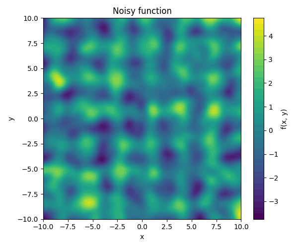
A function you can test your optimizer on
import numpy as np
from scipy.ndimage import gaussian_filter
from scipy.interpolate import RegularGridInterpolator
import matplotlib.pyplot as plt

def make_noisy_function(n=2, noise_amp=1.0, sigma=10,
                        xlim=(-10,10), ylim=(-10,10),
                        resolution=500):
    # This function takes as argument some optional parameters
    # and returns a Python function. So if you run `f = make_noisy_function()`
    # then f will become a function of two variables, i.e., `f(x,y)`.
    # This is an interesting function to minimize.

    # Base grid
    x = np.linspace(*xlim, resolution)
    y = np.linspace(*ylim, resolution)
    X, Y = np.meshgrid(x, y)

    # Base function
    Z = np.sin(n*X) + np.sin(n*Y)

    # Smooth noise
    noise = np.random.randn(*Z.shape)
    smooth_noise = gaussian_filter(noise, sigma=sigma)
    smooth_noise /= np.max(np.abs(smooth_noise))  # normalize to [-1,1]

    # Add noise
    Z_noisy = Z + noise_amp * smooth_noise

    # Interpolator turns it into a callable function f(x, y)
    f_interp = RegularGridInterpolator((x, y), Z_noisy, bounds_error=False, fill_value=None)

    def f(x, y):
        x = np.atleast_1d(x)
        y = np.atleast_1d(y)
        pts = np.column_stack([x, y])
        vals = f_interp(pts)
        if vals.size == 1:
            return vals.item()
        else:
            return vals

    return f

# Use the above constructor to make a function:
f = make_noisy_function(n=2, noise_amp=4.1, sigma=12)

# You may now use the above function in your code.

# Illustrate the function you have just made to visually identify minimia/maxima.

# Create a grid of points
x = np.linspace(-10, 10, 400)
y = np.linspace(-10, 10, 400)
X, Y = np.meshgrid(x, y)

# Evaluate your noisy function over the above grid.
Z = f(X.ravel(), Y.ravel()).reshape(X.shape)

# Plot
plt.figure(figsize=(6,5))
contour = plt.contourf(X, Y, Z, levels=40)
plt.colorbar(contour, label='f(x, y)')
plt.title('Visualize Noisy function')
plt.xlabel('x')
plt.ylabel('y')
plt.tight_layout()
plt.show()
This should produce a function like this:
Lec 11.1, Tue, Nov 18
Interpolate these points: download file
Lec 11.2, Thu, Nov 20
Curve-fit these points: download file