**E21 Lab 5: Rootfinding with Raytracing and Raymarching**
**[ENGR 21 - Fall 2026](../labs.html)**
**November 16-December 3, 2026**
**Due on Moodle prior to your next lab meeting.**
Your tasks for this lab will be to implement the Durand-Kerner method
for finding the roots of a polynomial, to implement a distance
function suitable for raymarching, and to extend the functionality
provided by the starter code in a direction of your choosing.
 to see an interactive version.](images/lab5_example1.jpg style="width: 75%")
(#) Objectives
Here are key skills you will develop in this lab:
* Implement an iterative root finding method not covered in lecture.
* Understand the connection between root finding and visible
surface determination in computer graphics.
* Represent images as arrays and form them by iterating a
mathematical function over each pixel (row, column) location.
* Gain appreciation for the fundamental connections between algebra
and geometry.
(##) Report Template
Use the provided [lab report template](https://docs.google.com/document/d/19ukWdXDg1bx2yTEAhnOS1yZyLL66wsPUvq-PM0dA1JU/copy) to answer the questions for this lab. For all E21 labs, please make sure to write up your answers to the questions in each exercise before you move on to the next task. The questions are designed to help you complete the labs efficiently.
# Background
Starter code for this lab is available [here](lab5.zip).
I'm assuming you all will be familiar with complex numbers before we
begin this lab.
## Digital representation of images
Commonly in computer graphics, we use 3D arrays of shape `(h, w, 3)` to represent RGB images with $h$ rows and $w$ columns.
Using the
[RGB color model](https://en.wikipedia.org/wiki/RGB_color_model), we
specify the color of a pixel using a combination of red, green, and
blue intensities -- hence three intensity values for each row/column
location in the image.
When using floating point formats to represent intensities, they are
usually scaled to the unit interval $[0.0, 1.0]$ with 0.0 being minimum intensity and 1.0 being maximum.
More frequently, images are represented using unsigned integer formats.
For an unsigned 8-bit integer, minimum intensity per channel is zero and maximum intensity is 255.
The `hello_image.py` program in the starter code shows how a spatially
varying signal can be used to fill up a numpy array with pixel
intensity values. It results in the `test.png` image shown below.

## Raytracing
!!! WARNING
Disclaimer: This section and the next one assume some knowledge of linear algebra,
specifically properties of dot products of vectors. If you haven't
seen the relevant course material, no worries!
The important take-away from the discussion below is that
**finding the intersection point of a view ray
and an analytic surface such as a sphere or a torus
can be accomplished by finding the roots of a particular polynomial.**
In computer graphics, [*ray tracing*]("https://en.wikipedia.org/wiki/Ray_tracing_(graphics)") refers to the process of image
formation by constructing a series of geometric rays originating from
a simulated camera that pass through the center of pixel locations on
a virtual image plane in front of the camera, as shown in the diagram below.
)](images/raytrace-wikipedia.png style="width: 75%")
Each ray is specified by its origin vector $\mathbf{r}_o \in \mathbb{R}^3$ and its
direction vector $\mathbf{r}_d \in \mathbb{R}^3$.
In general, all rays share a common origin which is
the position of the eye or the camera; however, each ray has its own
unique ray direction determined by its pixel location in the image.
The position of any point $\mathbf{p} \in \mathbb{R}^3$ along a given ray is given by
the parametric function $\mathbf{p}(t) = \mathbf{r}_o + t \, \mathbf{r}_d$, or
to examine the elements of each vector individually:
$$ \left[ \begin{array}{c} p_x \\ p_y \\ p_z \end{array} \right] =
\left[ \begin{array}{c} o_x \\ o_y \\ o_z \end{array}\right] + t \,
\left[ \begin{array}{c} d_x \\ d_y \\ d_z \end{array}\right].$$
Equivalently, you can conceptualize the vector equation
above as three coupled scalar functions
$$
\begin{align*}
p_x(t) & = o_x + t \, d_x \\
p_y(t) & = o_y + t \, d_y \\
p_z(t) & = o_z + t \, d_z. \\
\end{align*}
$$
In either case, the parameter $t$ corresponds to the distance traveled
along the ray. When $t = 0$, the point is at the origin, and as $t
\rightarrow \infty$, the point moves further and further along the ray
away from the origin in the direction of travel.
Determining whether each ray hits a primitive (such as a sphere or a
torus), and which surface has been hit first, can be accomplished
by finding the roots of a particular function of $t$.
In many cases, graphics primitives can be represented as
[implicit functions](https://en.wikipedia.org/wiki/Implicit_function)
where the surface of the object is the set of all points $\mathbf{p}$
such that $f(\mathbf{p}) = 0$.
For example, a sphere centered at the origin with radius $r$ is the
set of points $(x, y, z)$ such that
$$ x^2 + y^2 + z^2 = r^2.$$
We can define this as an implicit function by moving the radius term
to the left hand side:
$$ f(x, y, z) = x^2 + y^2 + z^2 - r^2 = 0. $$
We can also write this in vector form:
$$ f(\mathbf{p}) = \| \mathbf{p} \|^2 - r^2 = \mathbf{p} \bullet \mathbf{p} - r^2 = 0. $$
What's the connection to root finding? Let's substitute in our parametric equation for $\mathbf{p}(t)$ from above, and expand:
$$
\begin{align*}
0 & = \mathbf{p(t)} \bullet \mathbf{p(t)} - r^2 \\
& = (\mathbf{r}_o + t \, \mathbf{r}_d ) \bullet (\mathbf{r}_o + t \, \mathbf{r}_d ) - r^2.
\end{align*}
$$
Owing to the distributive and commutative products of the dot product, we can further transform
this equation:
$$
\begin{align*}
0 & = \mathbf{r}_o \bullet \mathbf{r}_o +
\mathbf{r}_o \bullet ( t \, \mathbf{r}_d ) +
( t \, \mathbf{r}_d ) \bullet \mathbf{r}_o +
(t \, \mathbf{r}_d) \bullet (t \, \mathbf{r}_d) -
r^2 \\
& = \mathbf{r}_o \bullet \mathbf{r}_o +
t \, \mathbf{r}_o \bullet \mathbf{r}_d +
t \, \mathbf{r}_d \bullet \mathbf{r}_o +
t^2 \, \mathbf{r}_d \bullet \mathbf{r}_d -
r^2 \\
& = \mathbf{r}_o \bullet \mathbf{r}_o +
t \, \mathbf{r}_o \bullet \mathbf{r}_d +
t \, \mathbf{r}_o \bullet \mathbf{r}_d +
t^2 \, \mathbf{r}_d \bullet \mathbf{r}_d -
r^2 \\
& = \mathbf{r}_o \bullet \mathbf{r}_o +
2 t \, \mathbf{r}_o \bullet \mathbf{r}_d +
t^2 \, \mathbf{r}_d \bullet \mathbf{r}_d -
r^2.
\end{align*}
$$
Grouping terms by order of exponent in $t$, we arrive at the quadratic equation
$at^2 + b t + c = 0$, where
$$
\begin{align*}
a & = \mathbf{r}_d \bullet \mathbf{r}_d \\
b & = 2 \mathbf{r}_o \bullet \mathbf{r}_d \\
c & = \mathbf{r}_o \bullet \mathbf{r}_o - r^2.
\end{align*}
$$
Note that a given ray can intersect a sphere at 0 points (misses the
sphere), 1 point (touches the sphere at a tangent point) or 2 points
(goes into, and then out of the sphere). Thes correspond to the
quadratic polynomial having 0, 1, or 2 real roots, respectively.
In the case of multiple real roots, we are always concerned with
finding the one that has the minimum $t$ because this is the first
point on the sphere that will be visible along the ray.
The implicit equation for a torus with minor radius $r_1$ and major radius $r_2$ is given by
$$ \left( r_2 - \sqrt{x^2 + y^2} \right)^2 + z^2 - r_1^2 = 0.$$
By an analogous procedure to a sphere, the ray-torus intersection
problem can be converted to finding the smallest real root of a
quartic (fourth-degree) polynomial.
!!! Tip
Numpy provides polynomial root finding via
[**`np.polynomial.polynomial.polyroots`**](https://numpy.org/doc/stable/reference/generated/numpy.polynomial.polynomial.polyroots.html).
Note that it expects coefficients to be provided in **increasing
order of exponent**, with constant term first, so that the
coefficients for the quadratic above would be specified as
`[c, b, a]`.
You will replace the starter code's calls to the numpy solver with your
own implementation of the Durand-Kerner method.
## Durand-Kerner method
The Durand-Kerner method is an iterative root finding technique for
polynomials. It uses complex arithmetic, and can find both the real
roots and the complex roots of a given polynomial. You will implement
this method to find the roots of quadratic and quartic polynomials
that arise in raytracing (see section below).
Let $f(x)$ be a degree $n$ polynomial with $n + 1$ coefficients. The
Durand-Kerner method maintains a list of $n$ root estimates $x_1$ to
$x_n$. Since it is an iterative method, we will denote the estimate
for the $k^\text{th}$ root at the $i^\text{th}$ iteration as $x_{k,i}$.
The update rule for Durand-Kerner is given by
$$
x_{k,i+1} = x_{k,i} - \frac{f(x_{k,i})}{\displaystyle \prod_{j < k}( x_{k,i} - x_{j,i+1} ) \cdot \prod_{j > k}( x_{k,i} - x_{j,i} ) }.
$$
To provide a concrete example with $n = 3$, we would start with
initial root estimates $x_{1,1}$, $x_{2,1}$, and $x_{3,1}$, then use the updates
$$
\begin{align*}
x_{1,2} & = x_{1,1} - \frac{f(x_{1,1})}{(x_{1,1} - x_{2,1})(x_{1,1} - x_{3,1})} \\
\\
x_{2,2} & = x_{2,1} - \frac{f(x_{2,1})}{(x_{2,1} - x_{1,2})(x_{2,1} - x_{3,1})} \\
\\
x_{3,2} & = x_{3,1} - \frac{f(x_{3,1})}{(x_{3,1} - x_{1,2})(x_{3,1} - x_{2,2})}.
\end{align*}
$$
!!! Tip
Given a point $x$ and coefficients $c_k$ in increasing order of exponent (i.e. constant term first), you
can evaluate a polynomial using [**`numpy.polynomial.polynomial.polyval`**](https://numpy.org/doc/stable/reference/generated/numpy.polynomial.polynomial.polyval.html).
Iteration should continue until the approximate relative error $\varepsilon_{k,i}$ for all
root estimates $x_{k,i}$ is below a specified tolerance. The approximate
relative error is given by
$$
\varepsilon_{k,i} = \frac{|x_{k,i} - x_{k,i-1}|}{|x_{k,i}|}.
$$
For further information, I suggest you check out the
[Wikipedia page on Durand-Kerner](https://en.wikipedia.org/wiki/Durand%E2%80%93Kerner_method).
!!! Warning
When implementing Durand-Kerner, you do not need to store a 2D
array of root estimates (e.g. for all $k$ and $i$) -- a 1D array
(over $k$) is sufficient.
I suggest you use a set of nested **`for`** loops that updates
each root over each each iteration. You may need to use a
temporary variable to store each new root
estimate before you compute approximate relative error and then
update the array with the new root estimate.
## Raymarching
One alternative method to root finding on polynomials is raymarching,
also known as sphere tracing. Raymarching is an iterative process
that updates a current estimate of the ray intersection point over time.
The initial estimate is placed at or close to the ray origin $\mathbf{r}_o$.
Then, at each iteration, the distance from the current estimated intersection
point to the nearest feature in the scene is computed. The next update is
obtained by marching that distance forward along the ray from the current position,
as shown in this animation by Inigo Quilez:
)](images/lab5_anim.gif style="width: 75%")
In raymarching, the ray direction vector is typically normalized to
have unit length, so that $\| \mathbf{r}_d \| = 1$. Then the update
rule is given by
$$ t_\text{new} = t_\text{old} + \mathrm{dist}\big(\mathbf{p}(t_\text{old})\big)
= t_\text{old} + \mathrm{dist}\big( \mathbf{r}_o + t_\text{old} \, \mathbf{r}_d \big) $$
where $\mathrm{dist}(\mathbf{p})$ is the function that computes the
distance from the point $\mathbf{p}$ to the nearest point in the
scene.
Iteration continues until the distance is within a preset tolerance
(i.e. a true intersection has been reached) or until a preset number
of iterations has been reached (at which point the ray is presumed
to have missed the objects in the scene).
Inigo Quilez maintains a
[web page](https://iquilezles.org/articles/distfunctions/) listing
many helpful examples of commonly used distance functions. Note that
the code examples on that page are provided in GL Shading Language
(GLSL), which has slightly different syntax than the Python starter
code that I provide.
## Lighting and shadowing
Once a ray intersection point has been determined, [additional
calculations](https://en.wikipedia.org/wiki/Computer_graphics_lighting) can be performed to determine the appearance of the
surface at that point. These usually depend on the [surface normal]("https://en.wikipedia.org/wiki/Normal_(geometry)") at
the intersection point -- that is, the direction of the vector that is
perpendicular to the object at the point of intersection. The surface
normal can be obtained from an implicit function representation of the
surface when raytracing, or by evaluating the gradient (first
derivative) of the distance function when raymarching.
Shadowing can be computed by casting another ray from the intersection
point to nearby light sources. If the ray can travel uninterrupted to
the light source without intersecting another object, the original
intersection point is lit; otherwise, it is in shadow.
Detailed discussion of the calculations involved in lighting are out
of the scope of this lab but I am happy to describe them during office hours!
# Lab exercises
Your team's job is to replace the call to numpy's polynomial solver
with your implementation of the Durand-Kerner method. You will then
implement a correct distance function to get the minimum distance from
any 3D point to the surface of a torus. Finally, you will extend the current
starter code to develop additional functionality of your choosing.
## Before you begin
Before you begin coding, look over the starter code with your partner,
then answer these questions.
(###) Questions
* **Q1)** *Note: more related to background material than code:*
Draw ray/torus intersections that correspond to finding 0, 1, 2,
and 4 real roots of the quartic polynomial (one drawing per case,
please). Include your drawings in your report PDF. You may
include photos/scans of **neat** hand drawings, or you can create
drawings in Google Slides, Canva, etc.
* **Q2)** In the **`smallest_positive_real_root`** function, what
is the purpose of the **`for`** loop? What is the purpose of
**`tol`** -- that is, why don't we just check to see if **`im ==
0`**?
* **Q3)** The **`test_roots`** function uses the **`assert`**
Python keyword. What does it do, and why might we use it? Cite
any sources you use to answer this question.
## Exercise 1
Modify the **`durand_kerner`** function in the starter code to provide
a correct implementation of the Durand-Kerner method.
If your implementation is incorrect, it will trigger an assertion
failure in **`test_roots`**.
!!! Tip
While you are completing your initial implementation, I suggest
you ignore the convergence criterion and simply iterate for a
large preset number of iterations (e.g. 1,000) until you
stop getting the assertion failure. Then, you can work on
halting when the approximate relative error criterion is
met for all root estimates.
Note that the runtimes for the numpy polynomial solver and your Durand-Kerner implementation may differ substantially. That's fine!
(###) Questions
* **Q4)** Regarding the **`guess_roots()`** function, how are the
initial guesses distributed in the complex plane? (It may help to
consider their angle/"complex argument" and magnitude.) Relate
this function to suggestions about initial values in the linked
[Wikipedia article](https://en.wikipedia.org/wiki/Durand%E2%80%93Kerner_method).
## Exercise 2
The current implementation of **`torus_distance`** does not compute
the minimum distance to the surface of a torus; instead it computes
the distance to a pill-shaped object. You should replace it with
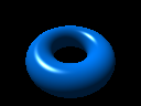
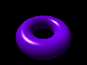
the correct torus distance function so that the shapes depicted
in `torus_trace.png` and `torus_march.png` match closely.
!!! Tip
You might find it helpful to follow these steps:
- Given an input point $\mathbf{p} = (x, y, z)$, project it to
the point $\mathbf{p}' = (x, y, 0)$ on the $xy$ plane.
- Get the closest point $\mathbf{p}_c$ to $\mathbf{p}'$ that
lies on the circle of radius $r_2$ around the origin in the $xy$ plane;
this is given by $\mathbf{p}_c = \mathbf{p}' \cdot r_2 \, / \, \| \mathbf{p}' \|$.
- The closest point on the torus to $\mathbf{p}$ is then the
same as the closest point to $\mathbf{p}$ on the surface of a
sphere centered at $\mathbf{p}_c$ with radius $r_1$.
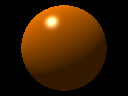
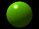
When you have finished task 2, you should have outputs that match
these four images:
## Exercise 3
Extend the program's functionality by choosing one of the following options:
- ***Easier*** - draw a different primitive (cone/octahedron/box/etc.)
- ***Medium*** - use raymarching to compose two objects next to each other (i.e. raytrace a sphere nested within a torus)
- ***Medium*** - replace the lighting computations with another coloring method (i.e. color by surface normal)
- ***Harder*** - use raymarching to perform set operations on objects (i.e. Boolean intersection of a cube and a sphere; Boolean difference of a cube and a sphere)
Or, choose another task you are interested in (but ask me first)!
(###) Question
* **Q5)** Describe your approach to exercise 3. How did you figure
out what code you needed to write, and how did it go?
# Lab report
Prior to your next lab meeting, submit a PDF writeup using
[the provided template](https://docs.google.com/document/d/19ukWdXDg1bx2yTEAhnOS1yZyLL66wsPUvq-PM0dA1JU/copy) with your names and answers to all questions
**Q1-Q5** above as well as the ones below:
* **Q6)** Copy your completed `lab5.py` to Google drive and share
it with my Swarthmore email address
([mzucker1@swarthmore.edu](mailto:mzucker1@swarthmore.edu)). Please be nice to my inbox and uncheck
“Notify people” when you share it. What is the URL (beginning
with https://) to your completed `lab5.py` file on Google drive?
* **Q7)** What problems did you run into when completing the tasks,
and how did you work together to overcome them?
* **Q8)** Compare and compast raytracing/raymarching. Does one
dominate the other (i.e. is one better in every possible
situation)? Does it matter if you use **`polyroots`**
vs. **`durand_kerner`**? Does it matter what types of shapes you
use?
* **Q9)** Did all group members contribute equally to all tasks?
If not, who did what for each exercise?
## Grading
Points will be assigned according to the following breakdown:
| Item | Grade value |
| :--- | --: |
| Answers to **Q1**-**Q9** and general writeup quality| 50% |
| Code for exercise 1 | 20% |
| Code for exercise 2 | 20% |
| Code for exercise 3 | 10% |