Lecture 17

E21 Computer Engineering Fundamentals

Emad Masroor

November 3, 2026

Another Approach to Solving Systems of Linear Equations

\[ \begin{bmatrix} A_{11} & A_{12} & A_{13} \\ A_{21} & A_{22} & A_{23} \\ A_{31} & A_{32} & A_{33} \end{bmatrix} \begin{bmatrix} x_1 \\ x_2 \\ x_3 \end{bmatrix} = \begin{bmatrix} b_1 \\ b_2 \\ b_3 \end{bmatrix} \]

Idea

\[ \begin{align*} A_{11}x_1 + A_{12}x_2 + A_{13}x_3 = b_1 &\implies {\color{red}{x_1}} = \frac{1}{A_{11}}(b_1 - A_{12}{\color{blue}{x_2}} - A_{13}{\color{blue}{x_3}}) \\[1ex] A_{21}x_1 + A_{22}x_2 + A_{23}x_3 = b_2 &\implies {\color{red}{x_2}} = \frac{1}{A_{22}}(b_2 - A_{21}{\color{blue}{x_1}} - A_{23}{\color{blue}{x_3}}) \\[1ex] A_{31}x_1 + A_{32}x_2 + A_{33}x_3 = b_3 &\implies {\color{red}{x_3}} = \frac{1}{A_{33}}(b_3 - A_{31}{\color{blue}{x_1}} - A_{32}{\color{blue}{x_2}}) \end{align*} \]

\({\color{blue}{x}}\): current value of \(x\)

\({\color{red}{x}}\): new value of \(x\)

Iterative vs. Direct Methods

  • An iterative solution to a system of equations \(Ax=b\) starts from a (usually arbitrary) guess and progressively improves the solution until the true solution is reached.

\[x^{(0)} \rightarrow x^{(1)} \rightarrow x^{(2)} \rightarrow \dots \rightarrow x^{(k)}\]

  • The ‘true’ answer is only reached in an approximate sense, but our approximate answer can be made as accurate as we would like — convergence.

  • Convergence is only guaranteed when the matrix \(A\) is nice.

  • In contrast, Direct methods like Gaussian Elimination + Substitution follow a procedure that takes us directly to the true answer (but could be more expensive)

The Jacobi Method

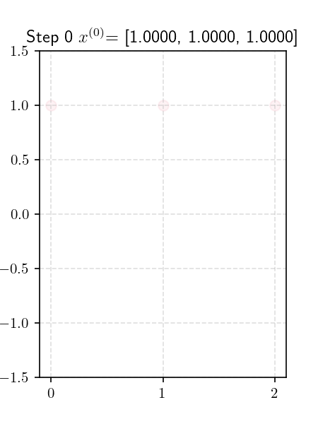
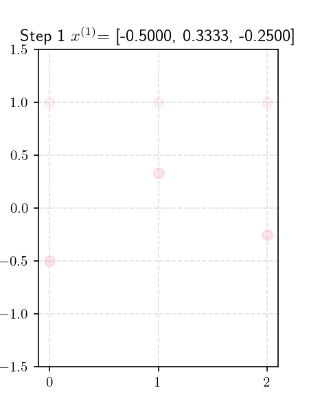
Use the worksheet to calculate a few steps of Jacobi’s method by hand/calculator to solve for the three components of the vector \(x\) in the following two systems.

System 1

\[ A = \begin{bmatrix} 4 & 1 & 2 \\ -\cfrac{1}{2} & 3 & \cfrac{3}{2} \\ 0 & 2 & 4 \end{bmatrix}, \quad b = \begin{bmatrix} 1 \\ 2 \\ 1 \end{bmatrix}, \quad \mathbf{x}^{(0)} = \begin{bmatrix} x_1^{(0)} \\ x_2^{(0)} \\ x_1^{(0)} \end{bmatrix} = \begin{bmatrix} 1 \\ 1 \\ 1 \end{bmatrix} \]
System 2

\[ A = \begin{bmatrix} -1 & 3 & 2 \\ 4 & 5/2 & -1 \\ 0 & 3 & 1 \end{bmatrix}, \quad b = \begin{bmatrix} 1 \\ 2 \\ 1 \end{bmatrix}, \quad \mathbf{x}^{(0)} = \begin{bmatrix} x_1^{(0)} \\ x_2^{(0)} \\ x_1^{(0)} \end{bmatrix} = \begin{bmatrix} 1 \\ 1 \\ 1 \end{bmatrix} \]
The Jacobi Method

\[ \begin{align*} x_1^{(k+1)} &= \frac{1}{A_{11}}\left( b_1 - A _{12} x_2^{(k)} - A_{13} x_3^{(k)} \right) \\ x_2^{(k+1)} &= \frac{1}{A_{22}}\left( b_2 - A _{21} x_1^{(k)} - A_{23} x_3^{(k)} \right) \\ x_3^{(k+1)} &= \frac{1}{A_{33}}\left( b_3 - A _{31} x_1^{(k)} - A_{32} x_2^{(k)} \right) \end{align*} \]

xnew[0] = 1/(A[0,0]) * (b[0] - A[0,1] * xold[1] - A[0,2] * xold[2])
xnew[1] = 1/(A[1,1]) * (b[1] - A[1,0] * xold[0] - A[1,2] * xold[2])
xnew[2] = 1/(A[2,2]) * (b[2] - A[2,0] * xold[0] - A[2,1] * xold[1])

Algorithm for Jacobi’s Method

\[x_j^{(k+1)} = \frac{1}{A_{jj}}\left( b_j - \sum^{N}_{i=1, \newline i \neq j} A_{ji} x_{i}^{(k)} \right)\]

Write Python code to implement this using three for loops

import numpy as np
import matplotlib.pyplot as plt

np.set_printoptions(4)
A = np.array([[4   ,1 ,2  ],
              [-1/2,3 ,3/2],
              [0   ,2 ,4  ]],dtype=np.float64)
b = np.array([1,
              2,
              1],dtype=np.float64)

xold = np.array([1,1,1],dtype=np.float64)
xnew = np.zeros(3)

n_steps = 3
for k in range(n_steps):
    # One for loop to go over each component of x
    for j in range(len(xold)):
        total = 0
        for i in range(len(xold)):
            if i != j:
                total += A[j,i] * xold[i]
        xnew[j] = (1/(A[j,j])) * (b[j] - total)
    print(xnew)
    xold = xnew.copy()

The need for copy

  • We often need a statement of the kind xold = xnew at the end of an iteration
  • The correct way to make this assignment is: xold = xnew.copy()
original = [1, 2, 3]

# "Make a copy" then append only to the new one
assigned = original
assigned.append(4)

print(f"Original (via =):     {original}") 
print(f"Assigned:             {assigned}")

# Make a copy using .copy() then append only to the new one
copied = original.copy()
copied.append(99)

print(f"\nOriginal (via .copy): {original}")
print(f"Copied:               {copied}")
Original (via =):     [1, 2, 3, 4]
Assigned:             [1, 2, 3, 4]

Original (via .copy): [1, 2, 3, 4]
Copied:               [1, 2, 3, 4, 99]

Saving History vs. overwriting

  • In direct methods, intermediate steps in the calculation are not meaningful.
  • In iterative methods, every iteration is a candidate solution
    • It is sometimes useful to save the solution history of iterative methods.

Overwrite each step

# First guess
xold = np.array([1.0,1.0,3.0])
xnew = np.zeros(3)

for i in range(10):
    # Perform one iteration, find xnew

    xold = xnew.copy()

Save history

# First guess
xold = np.array([1.0,1.0,3.0])
xnew = np.zeros(3)
xhst = np.zeros((10,3))

for i in range(10):
    # Perform one iteration, find xnew

    xhst[i,:] = xnew

Quantifying closeness of two numbers

We often want to know: ‘how far is \(x\) from a desired value \(x^*\)’.

  • For scalar real \(x\), this is measured by \[|x - x^*| = \sqrt{(x - x^*)^2}\]

  • For vector real \(\boldsymbol{x}\), \[\begin{align*} || \boldsymbol{x} - \boldsymbol{x}^* || &= \left| \left| \left(\begin{bmatrix} x_1 \\ x_2 \\ \vdots \\ x_n \end{bmatrix} - \begin{bmatrix} x^*_1 \\ x^*_2 \\ \vdots \\ x^*_n \end{bmatrix} \right) \right| \right| \\ &= \sqrt{(x_1 - x_1^*)^2 + (x_2 - x_2^*)^2 + ... + (x_n - x_n^*)^2} \end{align*}\]

  • More generally, the norm of an \(n\)-dimensional vector \(\boldsymbol{u} = \begin{bmatrix} u_1 \\ u_2 \\ \dots \\ u_n \end{bmatrix}\) is \(\sqrt{u_1^2 + u_2^2 + \dots + u_n^2}\)

The Residual vector and iterative methods

  • Iterative methods produce successive candidate solutions
  • If the method is good, the candidates should get better with more iterations
  • How do we define goodness of a candidate solution?
    • The equation \(A x = b\) can be used to numerically evaluate a candidate solution \(x^*\) by evaluating \(\boxed{\left| \left| b - A x^* \right| \right| }\)
    • This quantity is known as the (norm of the) residual corresponding to the candidate solution \(x^*\).
    • The smaller the (norm of the) residual, the better a candidate solution is.

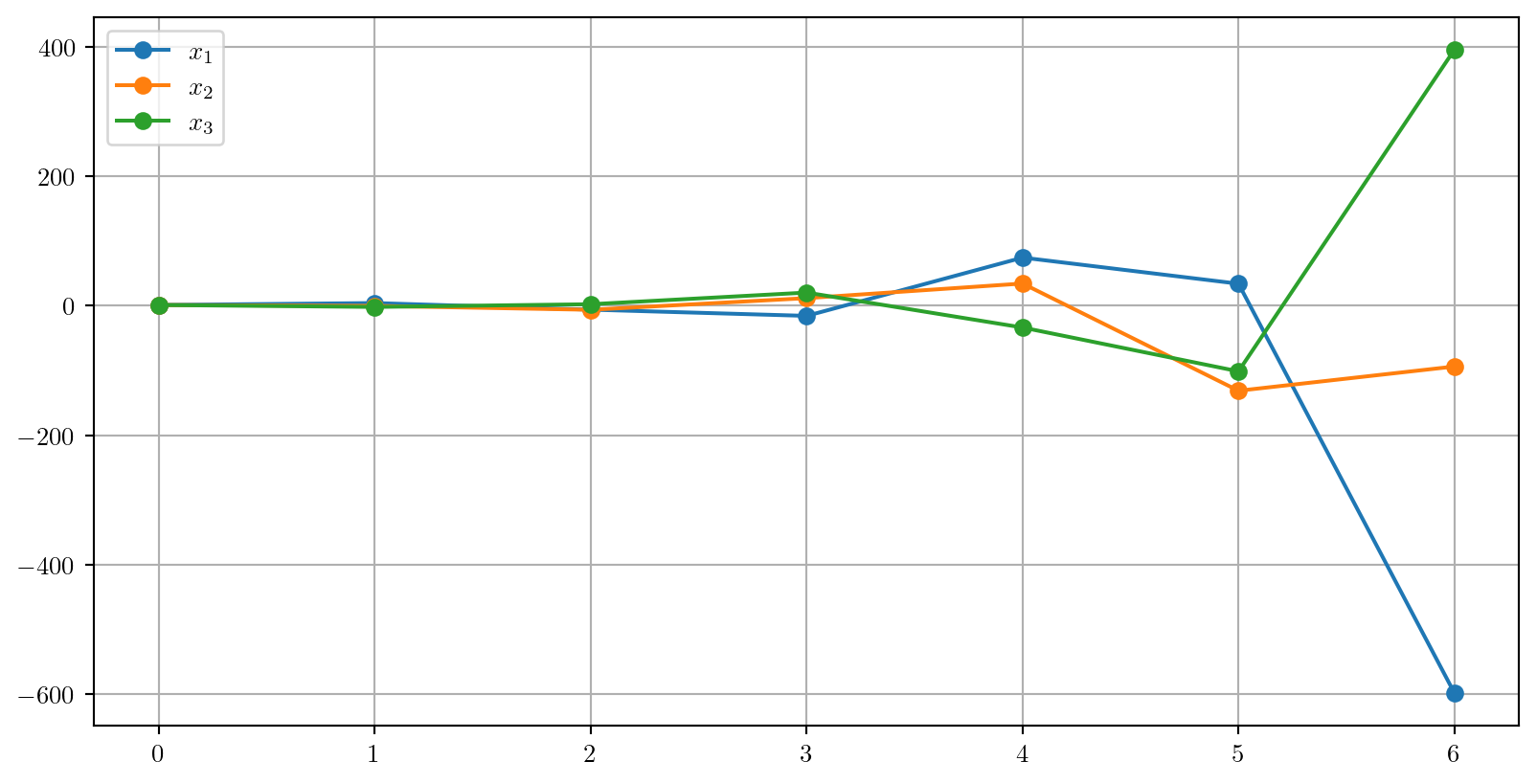
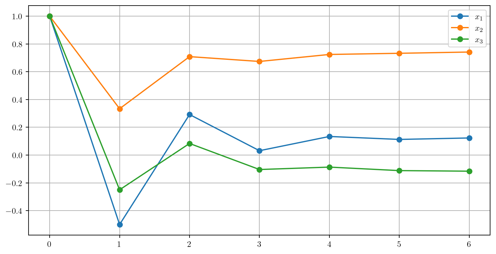
Divergence and Convergence

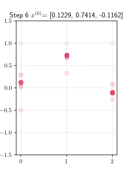
[ 4.  -0.4 -2. ]
[-6.2 -6.4  2.2]
[-15.8  11.6  20.2]
[ 74.2   34.16 -33.8 ]
[  33.88 -131.44 -101.48]
[-598.28  -94.    395.32]

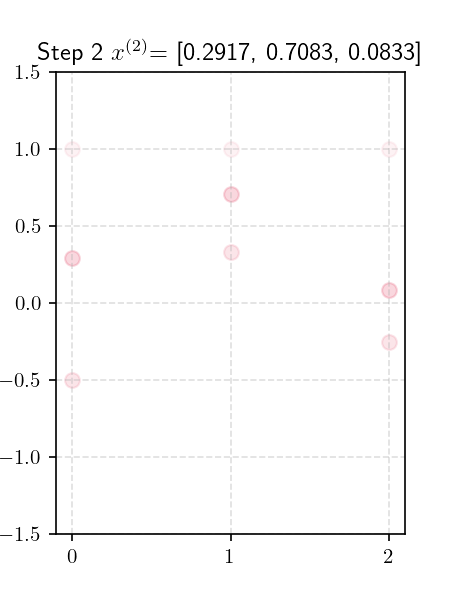
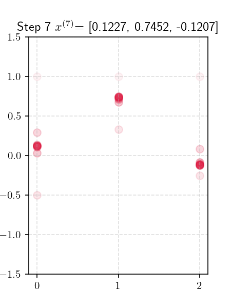
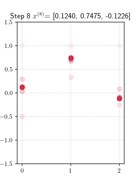
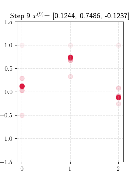
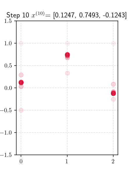
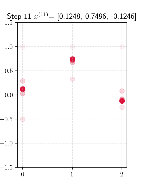
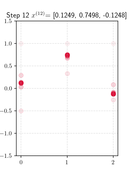
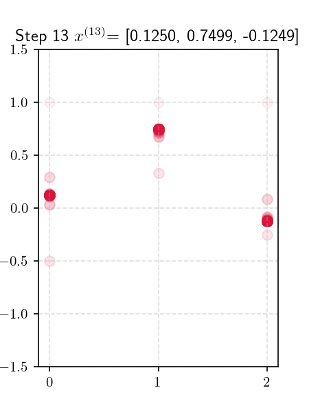
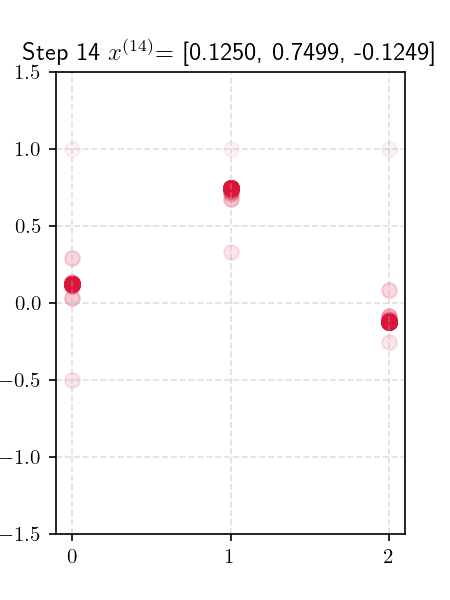
[-0.5     0.3333 -0.25  ]
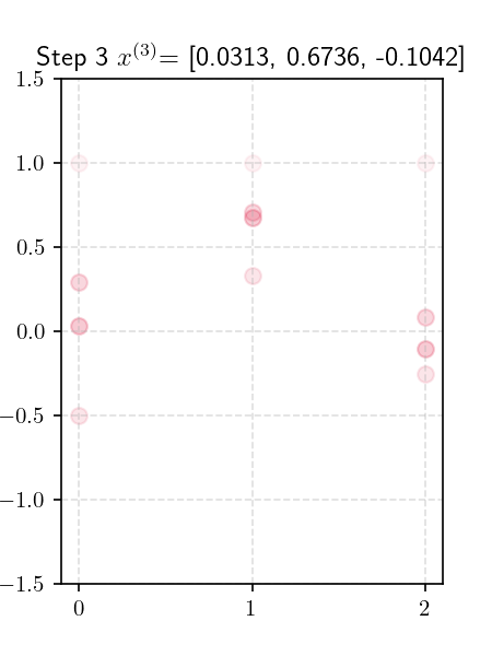
[0.2917 0.7083 0.0833]
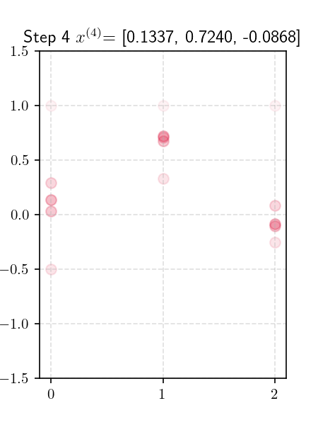
[ 0.0313  0.6736 -0.1042]
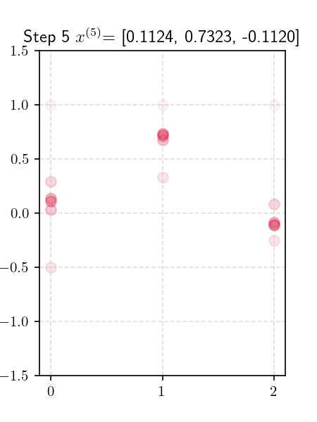
[ 0.1337  0.724  -0.0868]
[ 0.1124  0.7323 -0.112 ]
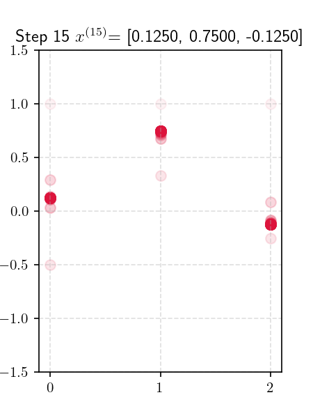
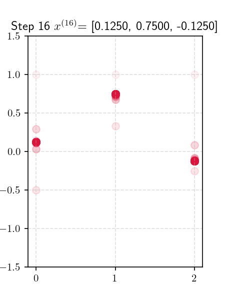
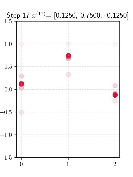
[ 0.1229  0.7414 -0.1162]

The Gauss-Seidel Approach

  • Gauss-Seidel is a slight modification to Jacobi’s method.
  • In Gauss-Seidel, we use the updated value on the right-hand side when available

Jacobi

\[ \begin{align*} {\color{red}{x_1^{(k+1)}}} &= \frac{1}{A_{11}}(b_1 - A_{12}{\color{blue}{x_2^{(k)}}} - A_{13}{\color{blue}{x_3^{(k)}}}) \\[1ex] {\color{red}{x_2^{(k+1)}}} &= \frac{1}{A_{22}}(b_2 - A_{21}{\color{blue}{x_1^{(k)}}} - A_{23}{\color{blue}{x_3^{(k)}}}) \\[1ex] {\color{red}{x_3^{(k+1)}}} &= \frac{1}{A_{33}}(b_3 - A_{31}{\color{blue}{x_1^{(k)}}} - A_{32}{\color{blue}{x_2^{(k)}}}) \end{align*} \]

Gauss-Seidel

\[ \begin{align*} {\color{red}{x_1^{(k+1)}}} &= \frac{1}{A_{11}}(b_1 - A_{12}{\color{blue}{x_2^{(k)}}} - A_{13}{\color{blue}{x_3^{(k)}}}) \\[1ex] {\color{red}{x_2^{(k+1)}}} &= \frac{1}{A_{22}}(b_2 - A_{21}{\color{red}{x_1^{(k+1)}}} - A_{23}{\color{blue}{x_3^{(k)}}}) \\[1ex] {\color{red}{x_3^{(k+1)}}} &= \frac{1}{A_{33}}(b_3 - A_{31}{\color{red}{x_1^{(k+1)}}} - A_{32}{\color{red}{x_2^{(k+1)}}}) \end{align*} \]

Niceness of the matrix \(A\)

  • Jacobi and Gauss-Seidel are guaranteed to converge if \(A\) is diagonally dominant.

Diagonal Dominance: if, for every row, the absolute value of the entry on the main diagonal (\(A_{11}, A_{22}\), etc.) is greater than the sum of the absolute values of all off-diagonal entries in that row, then the matrix is Diagonally Dominant.

  • Diagonal Dominance is a sufficient, but not necessary, condition for convergence of both Gauss-Seidel and Jacobi.