Lab 2: Stress-Strain Curves for Engineering Metals

Emad Masroor

Background

In actual engineering practice, tension tests of engineering metals are governed by standards such as the ASTM A370-26 Standard Test Methods and Definitions for Mechanical Testing of Steel Products. Although we will not be following this ASTM standard, it is an important reference for learning about how such tests are carried out in the field.

Typical stress-strain curves for ductile metals

Typical metals have a stress-strain curve that looks like this:

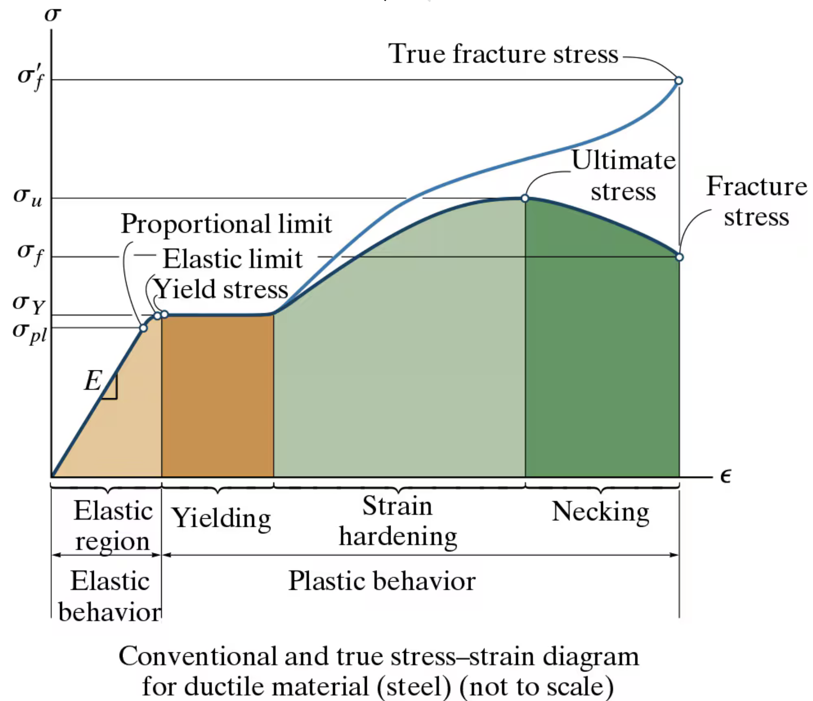
Another way to visualize stress-strain diagrams for metals is to use two different scales on the horizontal axis, as shown in Figure 1.

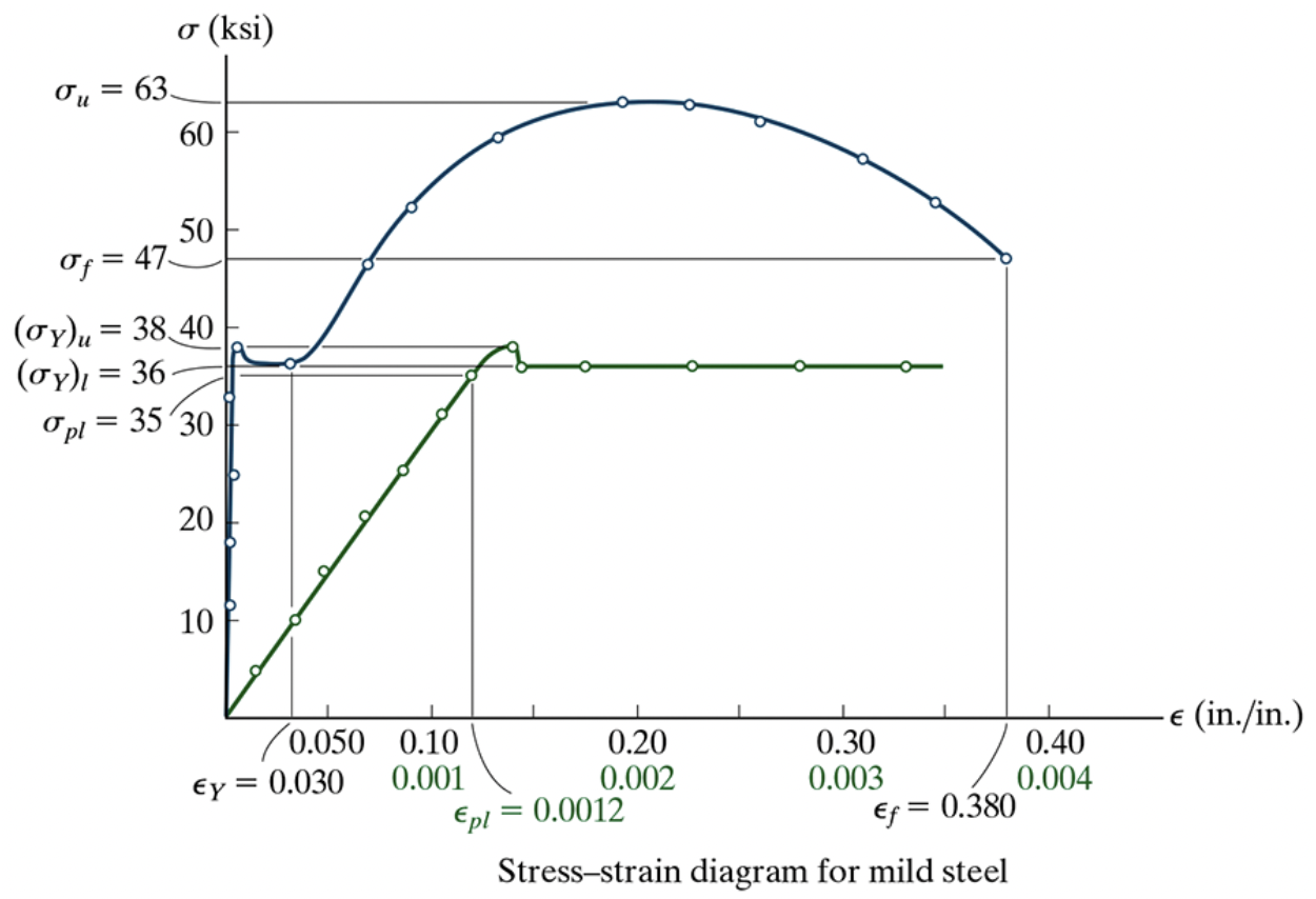
The 0.2% Offset Method

In order to decide when a metal has yielded, engineers use a rule called the 0.2% offset method. This rule states that a material can be said to have yielded under a load \(\sigma_Y\) when, after loading from \(\sigma = 0\) to \(\sigma = \sigma_Y\) and subsequently unloading to \(\sigma =0\), there is a residual strain of \(0.2 \%\) or \(0.002\).

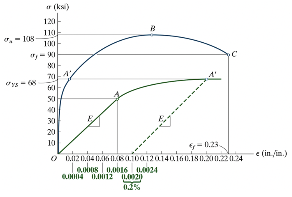
Figure 2: The 0.2% offset method graphically representend

It can be calculated by drawing a straight line parallel to the linear portion of the stress-strain curve, from a point on the nonlinear portion down to the strain axis. The line should intersect the strain axis at \(0.2 \%\); the intersection of this line with the stress-strain curve — point A’ above — is the yield point as determined by the \(0.2 \%\) method. This is illustrated in Figure 2.

Strain Energy Density

The area under a stress-strain curve is known as the strain energy density. It is positive when the sample is being loaded and negative when it is being unloaded.

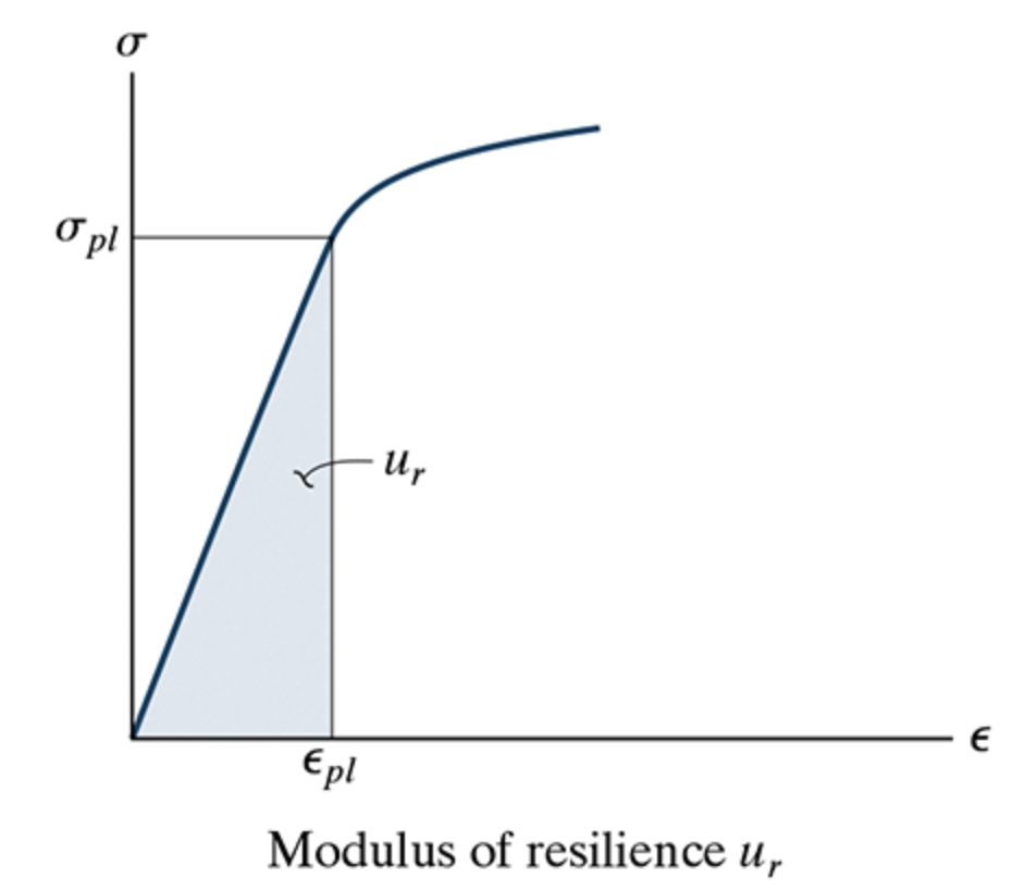
Modulus of Resilience

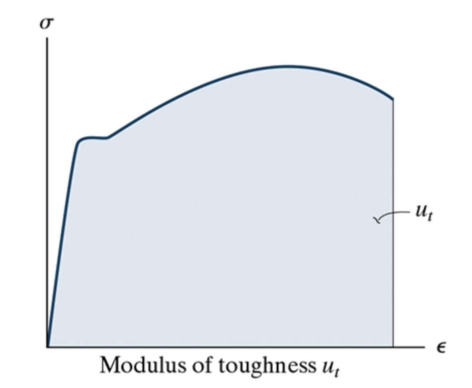
Modulus of Toughness

Trapezoidal Integration in MATLAB

MATLAB has two functions that are useful when calculating the area under a graph.

You should read the documentation of these functions to decide whether and how to use them for this lab.

Goal

Your overall goal in this lab is to produce high-quality stress-strain graphs for common engineering metals, annotating your graphs with material properties. Where applicable, these include:

The Young’s Modulus \(E\)
The proportional limit \(\sigma_{\text{pl}}\)
The yield stress \(\sigma_Y\)
The extent of the elastic region
The extent of the yielding region
The extent of the strain-hardening region
The extent of the necking region
The ultimate stress \(\sigma_u\)
The fracture stress \(\sigma_f\)
The modulus of toughness
The modulus of resilience

In practice, some of these quantities are difficult to distinguish from each other. A carefully-conducted tension test will help with this.

Sample List

Sample	Material	Quantity
ME-8231	Aluminum	2
ME-8243	Steel	2
AP-8223	0.005 in Brass (`648-07656`)	2
AP-8223	0.003 in Brass (`648-07653`)	2

Samples beginning with AP require the Materials Coupon Adapter

Preparation

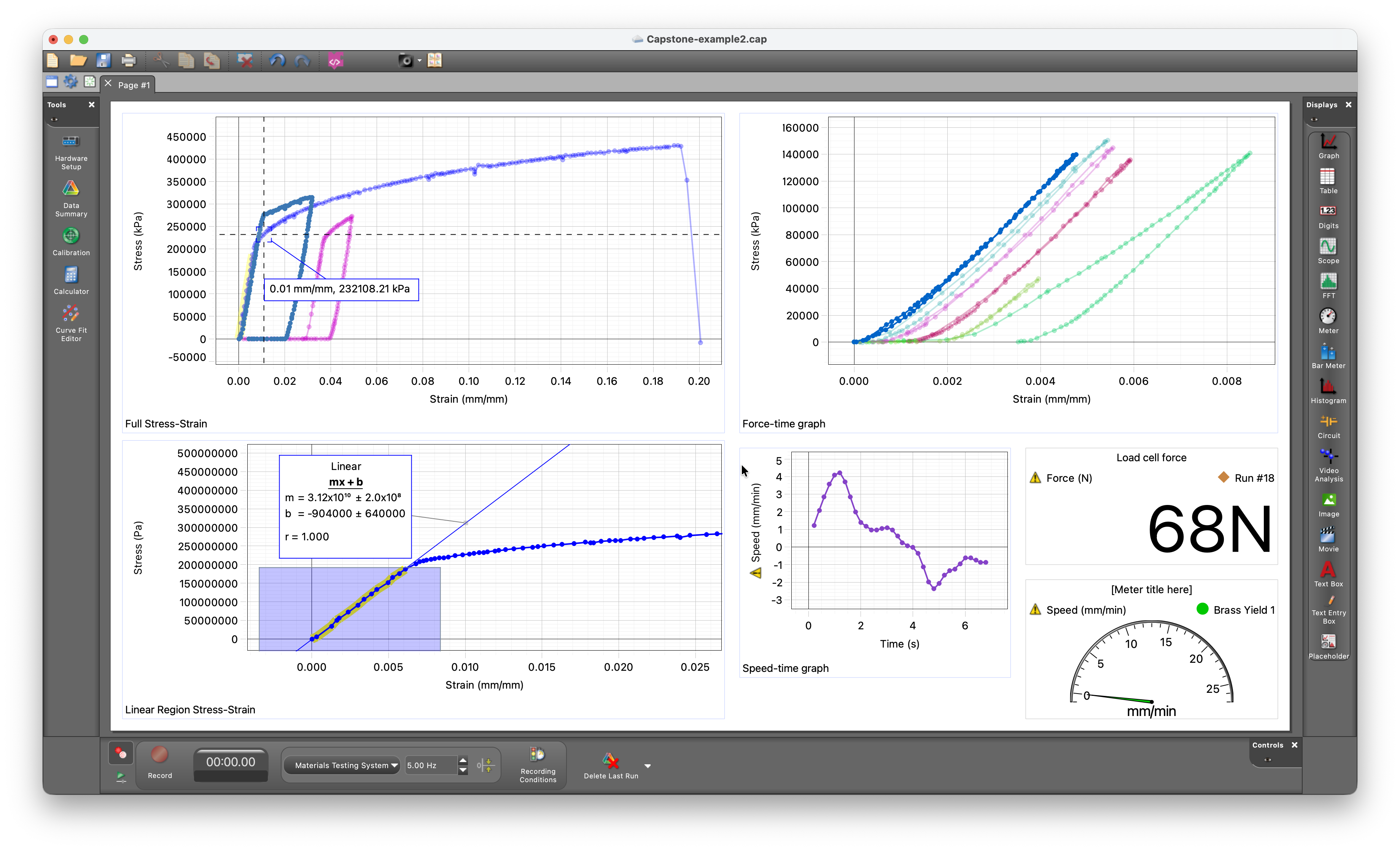
PASCO Capstone setup

For this lab, download the Capstone file located here. Save a copy of it, then delete all the data associated with it to replace it with your own data. You are encouraged to use a setup such as the following.

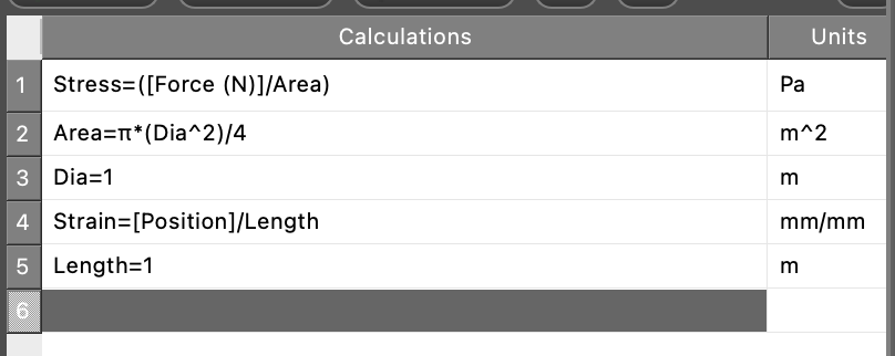
Prepare ‘Calculated Values’

Select the Calculator tab on the left panel of PASCO Capstone. This will be used to make ‘calculated values’, which are an additional feature of the software that allows you to visualize quantities that have been computed from the ones that the materials testing machine reports.

Note

You must put in correct values for the diameter and length of your sample.

Set up axes

You are encouraged to set up two sets of stress-strain axes.

On one set of axes, you should set up the horizontal axis to be primarily in the linear range of strains. This allows you to use the ‘Highlight range of points’ button and the ‘fit’ button to determine an approximate value for the Young’s Modulus, taking care to only include points in the linear range in your calculation.

On the other set of axes, your goal should be to capture the entire stress-strain curve with no zooming or panning required.

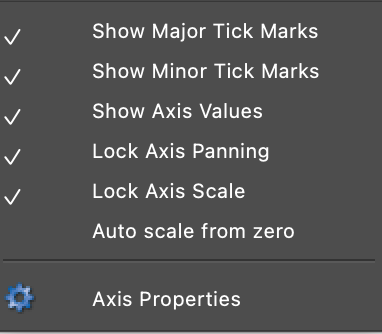
To help achieve this objectives, you should manipulate the axes as needed. You can also right-click each axis to make use of the following menu:

Loading at the right speed

The standard procedure for tensile testing engineering specimens involves a constantly-applied rate of displacement. Since this is not possible with the current apparatus, you must make an effort to apply displacements as slowly as you can, within the time constraints of the lab.

Note

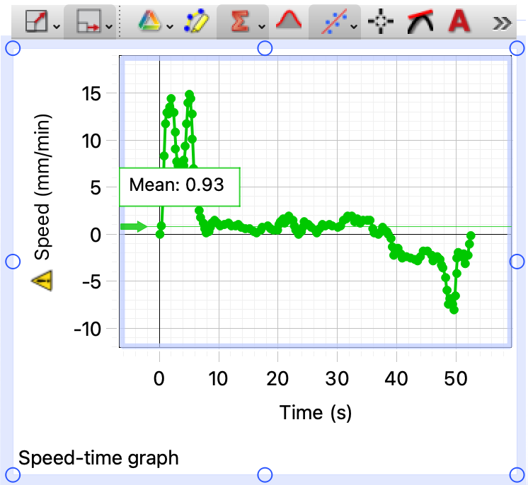
It is suggested that you use an average speed of 0.5 to 1.0 millimeter per minute. For every load cycle in this lab, you must record and later report the average speed at which loading / unloading was carried out.

☞ Calibration

For samples beginning with ME, you need to calibrate the machine in tension up to 7,000 N (and no more!) using the same procedure as lab 1.

For samples beginning with AP, you may need to recalibrate the machine to adjust for the smaller forces that will be observed.

Note

You may also directly use raw data instead. However, this may result in lower-quality data. Only do this as a last resort after consulting with the instructor.

Procedure

The following procedure must be followed for each sample in the above table.

☞ First specimen: Load to Failure

Slowly load the first specimen to failure. Save your Capstone project, and keep the data loaded in the system. Rename the ‘Run’ to keep track of the data later.

Note

You may want to keep this visible for the duration of your lab.

☞ Second specimen

The second specimen of each sample must be loaded in a particular manner, not directly to failure.

☞ Take measurements

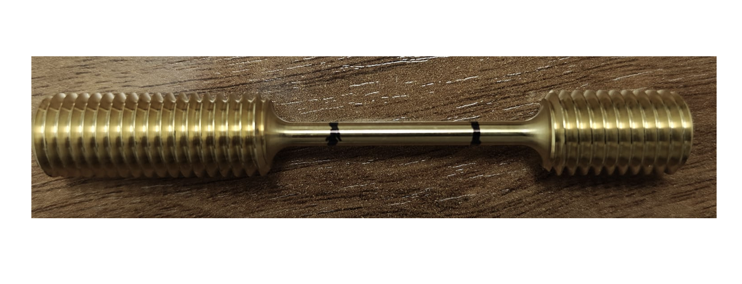
Place two marks on the second specimen using a Sharpie as shown below. Record the length of the portion of the specimen enclosed between the two marks using the calipers, taking care to use the appropriate precision in reporting the value that you find.

☞ Loading in the linear region

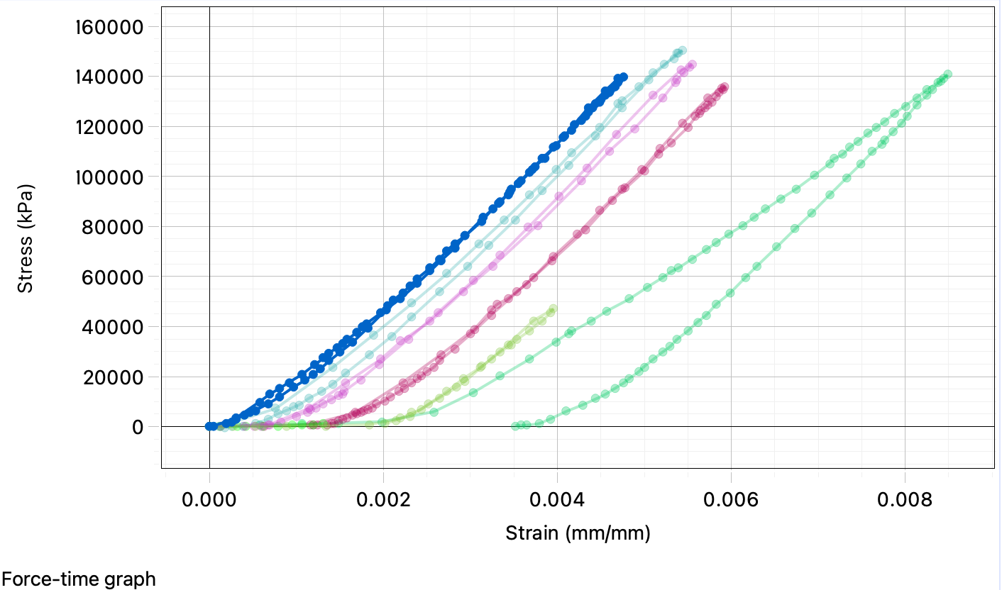
Carry out between 5 and 10 cycles of loading the sample from its completely unstressed state to some point before the yield point, i.e., only in the elastic region.

Warning

Do not let the material yield at this stage! You don’t have extra samples.

Your graphs should look approximately like the following.

Warning

Your graphs should all start from the origin if possible. Thus, some of the data runs above are examples of bad data collection. To start from the origin, you have to ensure that you have turned the crank up to the point of almost loading the specimen before clicking record.

If you don’t get this quite right, you can post-process later.

☞ Loading in the nonlinear region

Carry out between 5 and 10 cycles of loading + unloading in the plastic region of the stress-strain curve. As far as possible, try to do this without breaking the sample until the last cycle.

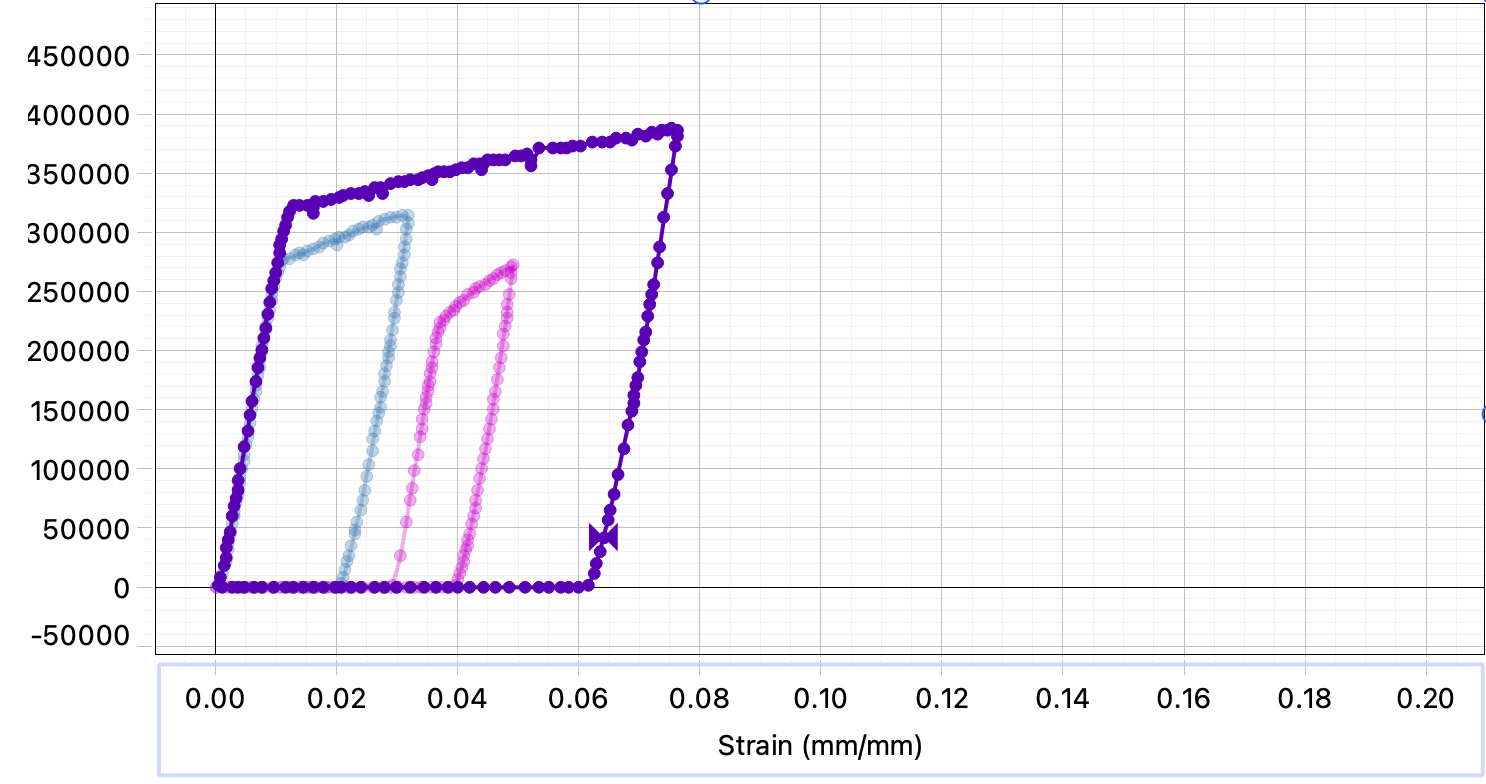
A ‘cycle of loading + unloading in the plastic region’ means that you should increase the displacement up to a certain value (i.e., load the sample) and then turn the crank in the reverse direction (i.e., unload the sample), all at a slow speed. You should ensure that you load the specimen past the point of yielding and also that you unload the specimen until it feels no more stress.

After each cycle, you should inspect the specimen and measure:

the smallest cross-sectional area anywhere on the specimen.
the length of the specimen between the two marks that you placed.

Note

Each loading cycle must apply a greater maximum strain than the last one. However, you should be careful to make small increments so as not to break the sample.

You can see an example of three cycles of loading followed by unloading in the following graph.

Data Analysis

The following data analysis should be carried out for each sample.

☞ Young’s Modulus

Use MATLAB’s curve-fitting toolbox to estimate the slope of the straight-line portion of the stress-strain graph.

Determine the value of Young’s Modulus for each sample using all of your experiments. How confident are you about this value? Use a box chart, sample below, to communicate your results. A box chart can be made in MATLAB using the boxchart function, which you should look up on the MATLAB documentation page.

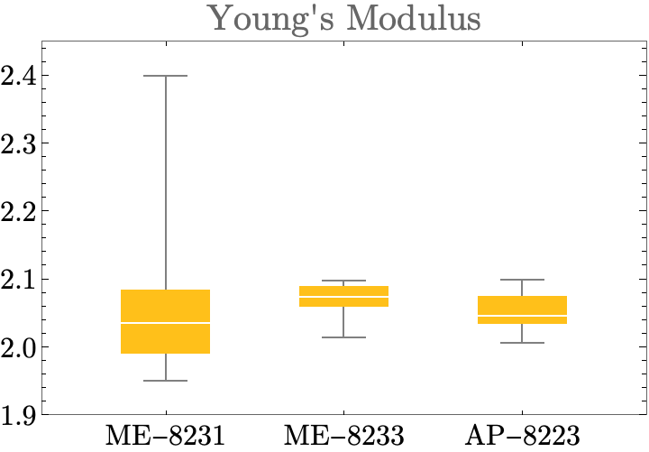
Figure 4: Sample Box Chart

☞ Strain Energy Density vs. subsequent Ultimate Stress

For loading in the nonlinear region, it is possible to calculate the maximum strain energy denisty stored in the specimen at the end of a tensile test that has pulled the specimen past the point of yield. This is equal to the area under a stress-strain curve loading curve, in the case of a monotonically-loaded specimen, and equal to the area between the loading and unloading curves in a specimen that is first loaded and then unloaded.

Using one of the two MATLAB functions listed above, calculate the strain energy density stored in the sample during each load-unload cycle. Use this information to make a table similar to Table 1 for each sample. In the ‘dimensions’ column, write down the length (of the region you marked) and the smallest cross-sectional area anywhere in the test region of the sample.

Table 1

Cycle No.	Ultimate Stress Reached	Strain Energy Density stored
0
1	\(100,000\) MPa	\(000\) (units)
2

How to fill this table

The first row of your table should be filled using the ultimate stress and strain energy density found by monotonically loading the first specimen.
The subsequent rows should be filled using the successive load-unload cycles on the second specimen.
The number of rows you have depends on the number of times you were able to load/unload the second specimen (between 5 and 10)
If fracture occurred, note that with an asterisk.
There should be one table like this for each of the four samples in this lab.

☞ Yield Strength using the 0.2% Offset Method

Calculate the yield strength of each sample using the 0.2% offset method. Illustrate the use of this method by showing a graph of stress vs. strain similar to OAAEO in Figure 2.

☞ Other Material Properties

Create a table with the following material properties.

Table 2

Property	Sample 1	Sample 2	Sample 3	Sample 4
Young’s Modulus
Yield Stress
Ultimate Stress
Fracture Stress
Modulus of Resilience
Modulus of Toughness

Memo

Write a memo reporting on your tension testing of the samples associated with this lab. You should structure your memo as a letter written to a client who asked you to characterize the properties of these four samples in the elastic and the plastic regime. In your memo, comment on how your testing procedure differs from the ASTM standard.

Your figures should be computer-generated in MATLAB, Python’s matplotlib, or similar.

You should be candid, in the narrative, about the degree of confidence you have in the numbers you are quoting to your client, and you should pay special attention to significant figures.

Part I: material properties

The following figures/charts will form the technical core of your memo, around which you should craft a professional narrative. This narrative should avoid the use of phrases such as “in this lab” or “we were given”, etc., and should instead focus on the client’s need for high-quality stress-strain diagrams and reliable values for the relevant properties.

For each sample, produce:

A global stress-strain curve for each sample
A stress-strain curve in the elastic region + the beginning of the plastic region, for each sample
A completed Table 2
An annotated version of the stress-strain graphs for each sample showing how the values above were calculated. See how to annotate plots in MATLAB here
A box chart of Young’s Moduli similar to Figure 4. There should be four entries in this box chart.

You may choose to combine 1 and 2 into a single figure, similar to Figure 1 by making creative use of MATLAB’s plotting facilities. For example, you can add a second horizontal axis to your figure.

Part II: Plastic behavior

In this part of the memo, you should reflect on the behavior of the samples in the plastic region of the stress-strain curve. You should quantify the amount of ‘strain hardening’ that was observed and comment qualitatively on how the true stress/strain would differ from the engineering stress/strain that has been reported here.

In particular, you should generate, for each sample,

a nicer-looking version of Figure 3 for each material, together with at least one illustration of the “area under the curve” approach to strain energy as applied to your data. For the loading-unloading figure, it is not necessary to include every cycle that you applied in your final figure.
Table 1, taking care to report your results in order of increasing maximum applied strain. For this table, you should include every cycle that you applied and note fracture if it occurred.

This part of your memo should explain to the client, in a quantiative and scientific manner, the changes they can expect to the material properties of their samples if they are loaded beyond the proportional/yield limit.