Numerical Solution of Initial Value Problems

Spring 2025 • E91 • Swarthmore College •

The Initial Value Problem

Numerically solve the initial value problem given by

\[\dot{y} = \sin y, \, y(0) = \pi/6.\]

Using Python

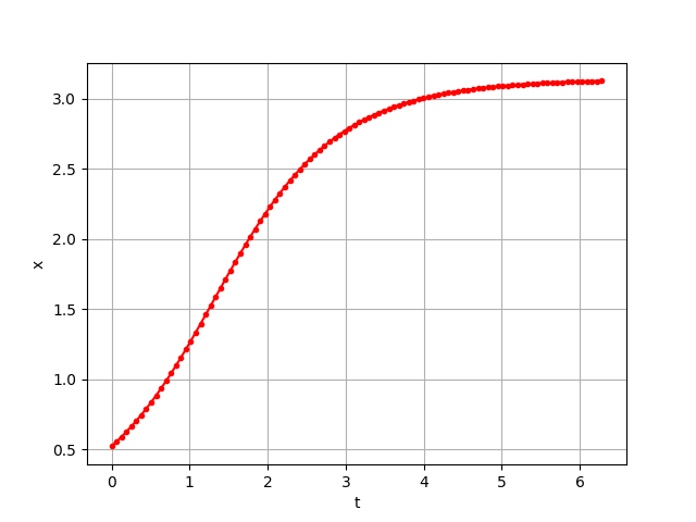
You must have the packages scipy, numpy, and matplotlib installed in order to use the import statements shown below. If you don’t know how to install these packages, please see the tutorial here.

from scipy.integrate import solve_ivp
import matplotlib.pyplot as plt
from numpy import array,exp,sin,pi,linspace

def f1(t,x):
    return sin(x)

x_init      = array([pi/6]) 
t_vector    = linspace(0,2*pi,100)
solution1   = solve_ivp(f1,                         # r.h.s of diff. eq
                        (t_vector[0],t_vector[-1]), # start & end time
                        x_init,                     # initial condition
                        t_eval=t_vector)            # times to plot

plt.figure(1)
plt.plot(solution1.t,solution1.y[0],'r.-')
plt.grid()
plt.xlabel('t')
plt.ylabel('x(t)')
plt.show()    # uncomment to preview figure

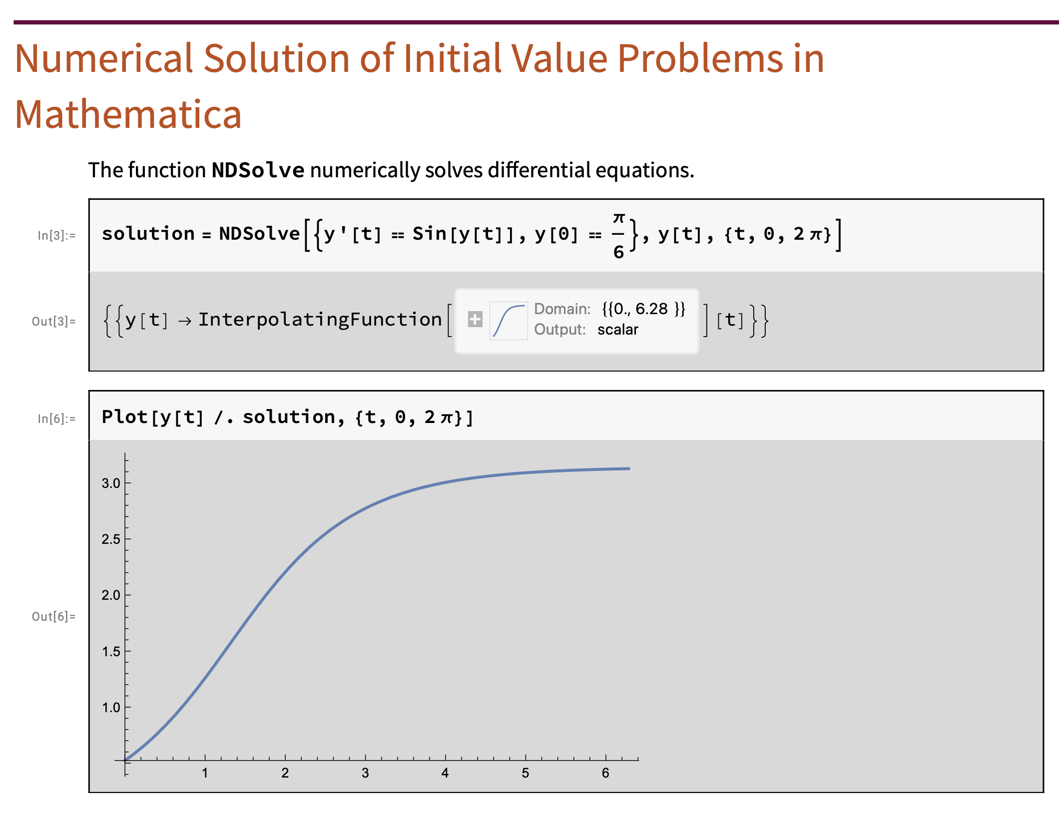
Using Mathematica

solution = 
 NDSolve[{y'[t] == Sin[y[t]], y[0] == \[Pi]/6}, y[t], {t, 0, 2 \[Pi]}]

Plot[y[t] /. solution, {t, 0, 2 \[Pi]}]

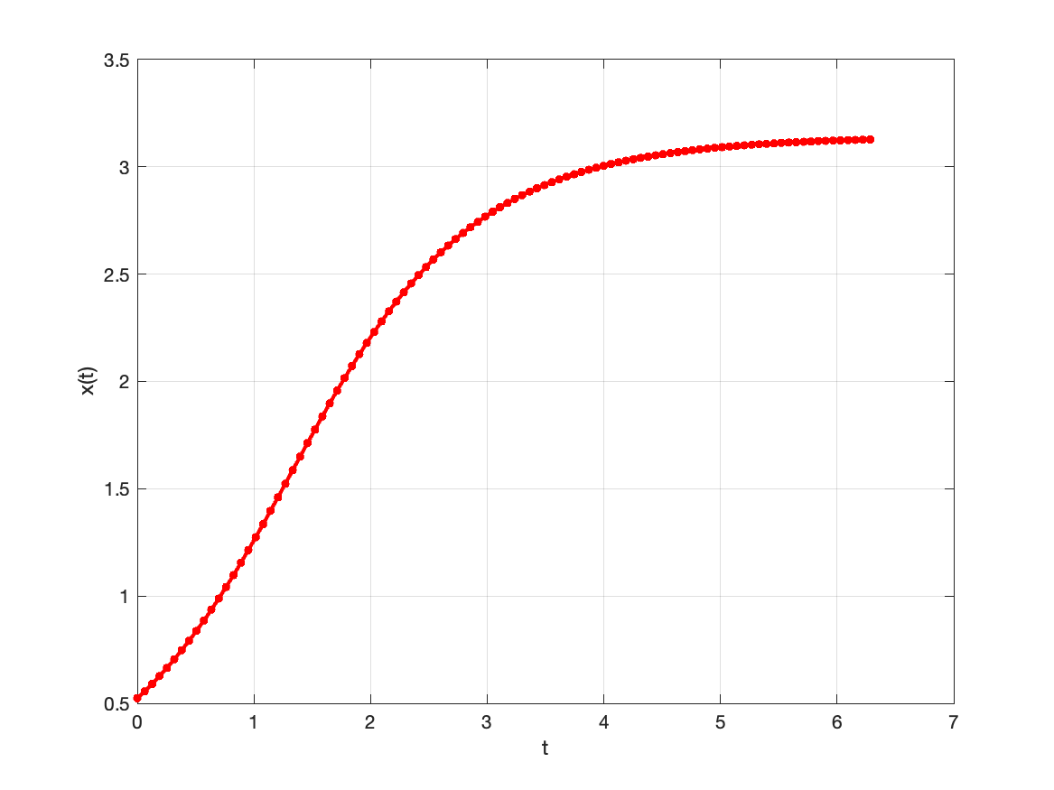
Using MATLAB

x_init      = pi/6;
t_vector    = linspace(0,2*pi,100);
[t,x]       = ode45(@rhs,t_vector,x_init);

figure(1);
plot(t,x,LineWidth=2,Marker=".",MarkerSize=12,Color='Red');
xlabel('t');
ylabel('x(t)');
grid on;

For this to work, you must have the file rhs.m in the same directory, and the file should contain:

function [dydt] = rhs(t,y)
dydt = sin(y);
end