Lecture 11
E12 Linear Physical Systems Analysis
February 24, 2026
The State Variable Approach
We often need to track more than one variable and its change.
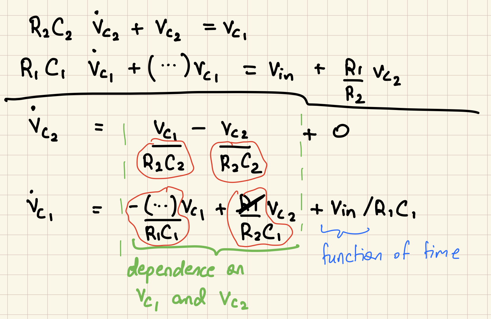
\[ \begin{aligned} R_2 C_2 \dot{v}_{c_2} + v_{c_2} &= v_{c_1} \\ R_1 C_1 \dot{v}_{c_1} + \left( 1 - \frac{R_1}{R_2}\right) v_{c_1} &= v_{\text{in}} + \frac{R_1}{R_2} v_{c_2} \end{aligned} \]
\[ \begin{aligned} R_2 C_2 \boxed{\dot{v}_{c_2}} + \boxed{v_{c_2}} &= \boxed{v_{c_1}} \\ R_1 C_1 \boxed{\dot{v}_{c_1}} + \left( 1 - \frac{R_1}{R_2}\right) \boxed{v_{c_1}} &= v_{\text{in}} + \frac{R_1}{R_2} \boxed{v_{c_2}} \end{aligned} \]
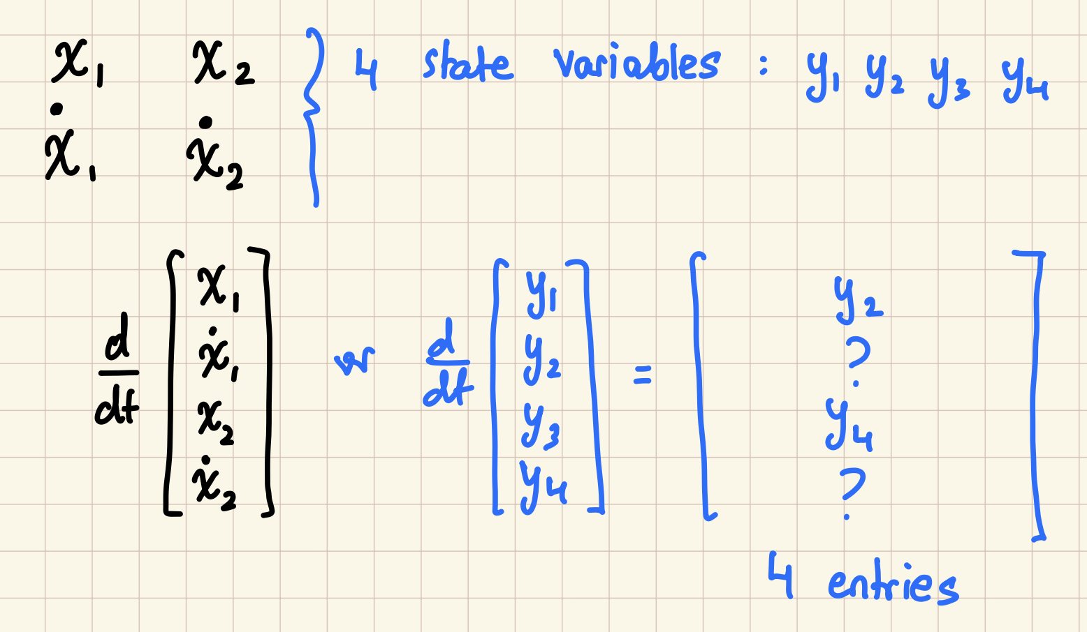
- Identify the variables whose change we are interested in (a.k.a state variables)
- Assemble into a vector: \[\begin{bmatrix} v_{c_1}(t) \\ v_{c_2}(t) \end{bmatrix}\]
- This vector is known as the state of the system at any given time \(t\)

Equivalent Notations for a system’s equations
Two individual equations \[ \begin{aligned} \dot{x}_1 &= f_1(x_1,x_2,t) \\ \dot{x}_2 &= f_2(x_1,x_2,t) \end{aligned} \]
One “vector equation” \[ \begin{bmatrix} \dot{x}_1 \\ \dot{x}_2 \end{bmatrix} = \begin{bmatrix} f_1(x_1,x_2,t) \\ f_2(x_1,x_2,t) \end{bmatrix} \]
One “vector equation” with explicit derivative \[ \frac{d}{dt} \begin{bmatrix} x_1 \\ x_2 \end{bmatrix} = \begin{bmatrix} f_1(x_1,x_2,t) \\ f_2(x_1,x_2,t) \end{bmatrix} \]
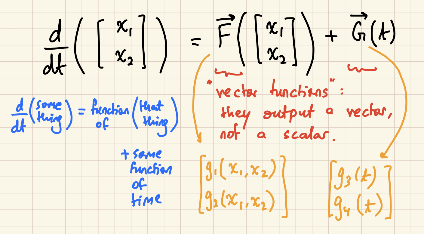
Vector symbols \[ \frac{d\boldsymbol{x}}{dt} = \begin{bmatrix} f_1(\boldsymbol{x},t) \\ f_2(\boldsymbol{x},t) \end{bmatrix}, \boldsymbol{x} = \begin{bmatrix} x_1 \\ x_2 \end{bmatrix} \]
Separating out the time-dependence \[ \begin{aligned} \dot{x}_1 &= g_1(x_1,x_2) + g_3(t) \\ \dot{x}_2 &= g_2(x_1,x_2) + \underbrace{g_4(t)}_{\text{known}} \end{aligned} \]
Using ‘vector functions’
![]()
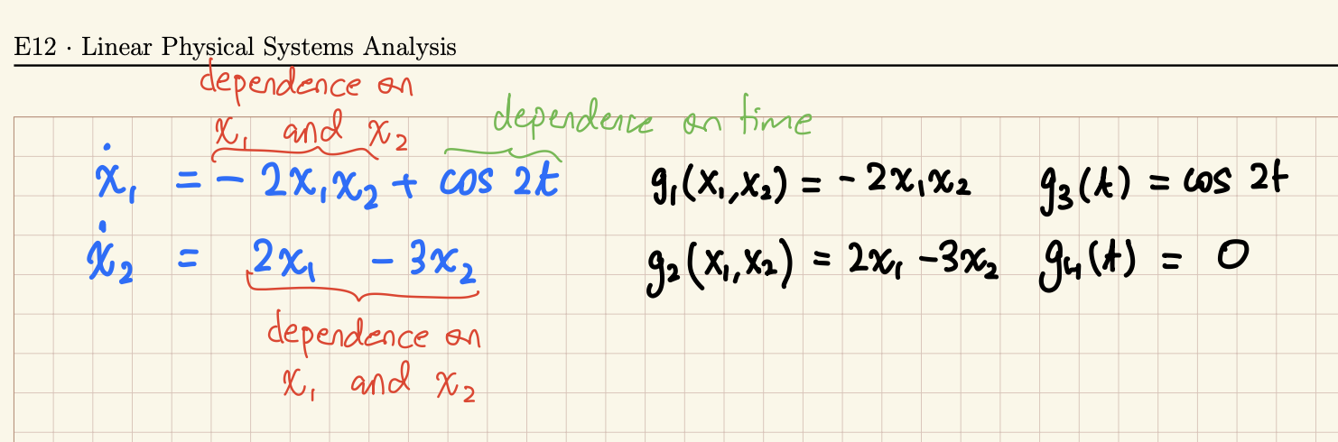
Example 1: State-variable form
Express the following system of equations
\[ \begin{aligned} \dot{x}_1 + 2 x_1 x_2 - \cos 2t &= 0 \\ \dot{x}_2 + 3 x_2 - 2x_1 &= 0 \end{aligned} \]
in the form of state-variable equations:
\[ \begin{aligned} \dot{x}_1 &= g_1(x_1,x_2) + g_3(t) \\ \dot{x}_2 &= g_2(x_1,x_2) + g_4(t) \end{aligned} \]
Explicitly specifying what \(g_1\), \(g_2\), \(g_3\) and \(g_4\) are.
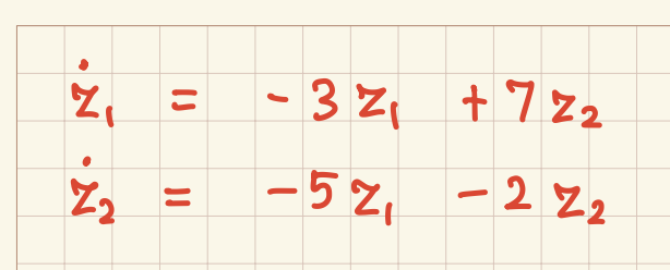
Example 2: State-variable form
Express the following system of equations
\[ \begin{aligned} \dot{z}_1 + 3 z_1 - 7 z_2 &= 0 \\ \dot{z}_2 + 2 z_2 + 5 z_1 &= 0 \end{aligned} \]
in the form of state-variable equations:
\[ \frac{d}{dt} \begin{bmatrix} z_1 \\ z_2 \end{bmatrix} = \begin{bmatrix} f_1(z_1,z_2,t) \\ f_2(z_1,z_2,t) \end{bmatrix} \]
Explicitly specifying what \(f_1\), \(f_2\) are.
Interpreting a system’s equations
\[ \begin{aligned} {\color{red}{R_2 C_2}} \color{blue}{\dot{v}_{c_2}} + \color{green}{v_{c_2}} &= \color{green}{v_{c_1}} \\ {\color{red}{R_1 C_1}} \color{blue}{\dot{v}_{c_1}} + {\color{red}{\left( 1 - \frac{R_1}{R_2}\right)}}\color{green}{v_{c_1}} &= \color{brown}{v_{\text{in}}} + \color{red}{\frac{R_1}{R_2}} \color{green}{v_{c_2}} \end{aligned} \]
- Constant parameters
- State variables
- Derivatives of state variables
- Input, forcing function, i.e. known functions of time
In Linear Physical Systems, the rate of change of the state variables depends linearly on the state variables.
Interpreting a system’s equations
\[ \begin{aligned} {\color{red}{R_2 C_2}} \color{blue}{\dot{v}_{c_2}} + \color{green}{v_{c_2}} &= \color{green}{v_{c_1}} \\ {\color{red}{R_1 C_1}} \color{blue}{\dot{v}_{c_1}} + {\color{red}{\left( 1 - \frac{R_1}{R_2}\right)}}\color{green}{v_{c_1}} &= \color{brown}{v_{\text{in}}} + \color{red}{\frac{R_1}{R_2}} \color{green}{v_{c_2}} \end{aligned} \]
Write these equations in state-variable form.
\[ \begin{aligned} \dot{x}_1 &= g_1(x_1,x_2) + g_3(t) \\ \dot{x}_2 &= g_2(x_1,x_2) + g_4(t) \end{aligned} \]
Explicitly specifying what \(x_1\), \(x_2\), \(g_1\), \(g_2\), \(g_3\) and \(g_4\) are.
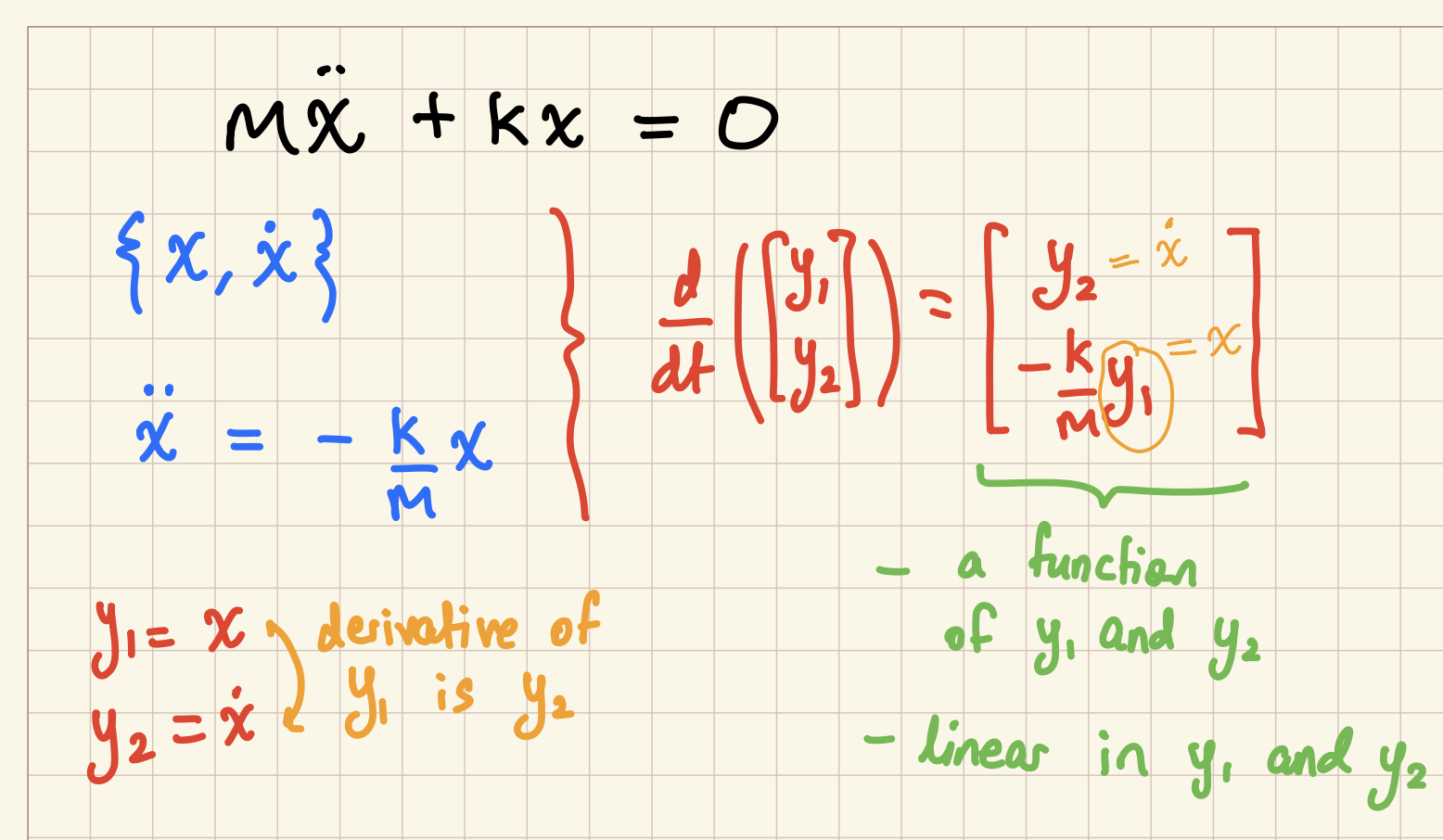
Example: A second-order equation in state-variable form
\[m \ddot{x} + k x = 0\]
Energy-storing elements and the order of a system
Recall circuits from HW 2

Typically: The order of a system = the number of state variables = the number of energy-storing elements
Energy-storing elements of a circuit

- Resistors dissipate energy
- Capacitors store energy in the form of separated charges
- Inductors store energy in the form of a magnetic field
| Element | Resistor | Capacitor | Inductor |
|---|---|---|---|
| Symbol | \(R\) | \(C\) | \(L\) |
| Stored Energy | \(0\) | \(\frac{1}{2} C v^2\) | \(\frac{1}{2} L i^2\) |
| Dissipated Power | \(v i = i^2 R = \frac{v^2}{R}\) | \(0\) | \(0\) |
| Form of Energy | Heat | Separated opposite charges | Magnetic Field due to current |
Energy-storing elements of a mechanical system
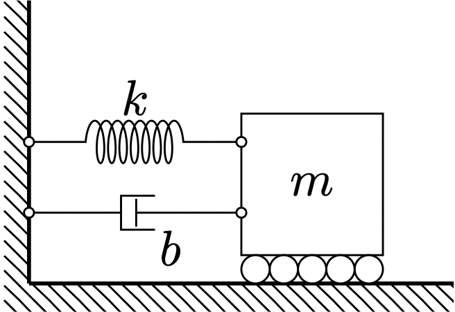
- Dampers/dashpots/frictionful surfaces dissipate energy
- Masses store kinetic energy when moving
- Springs store (elastic) potential energy when stretched or compressed
| Element | Damper | Spring | Mass |
|---|---|---|---|
| Symbol | \(b\) | \(k\) | \(m\) |
| Stored Energy | \(0\) | \(\frac{1}{2} k x^2\) | \(\frac{1}{2} m v^2\) |
| Dissipated Power | \(b v \times v = b v^2\) | \(0\) | \(0\) |
| Form of Energy | Heat | Potential Energy | Kinetic Energy |
Place equations in state-variable form
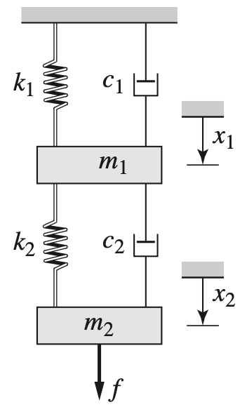
It is known that the governing equations for this system are: \[ \begin{aligned} 5 \ddot{x}_1 + 12 \dot{x}_1 + 5 x_1 - 8 \dot{x}_2 - 4 x_2 &= 0 \\ 3 \ddot{x}_2 + 8 \dot{x}_2 + 4 x_2 - 8 \dot{x}_1 - 4 x_1 &= f(t) \end{aligned} \]