Problem Set 2 Solutions
ENGR 12, Spring 2026.
Solutions
1 RC Circuit with constant input
Consider the circuit diagram shown below. The capacitor starts out with no charge across it, i.e., \(v_C=0\) at \(t=0\).

1.1 Voltage across capacitor and resistor
In class, we wrote down an equation for \(v_C(t)\).
Use this equation, and the circuit diagram, to plot, on the same set of axes, the voltage across the capacitor \(v_C(t)\) and across the resistor \(v_R(t)\) as a function of time for the first three seconds of the circuit’s operation. You must use correct units in your answer. Also write down a mathematical expression for these two curves, without using any arbitrary constants.
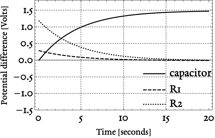
The following plot shows the evolution of voltage across the capacitor and the resistor.
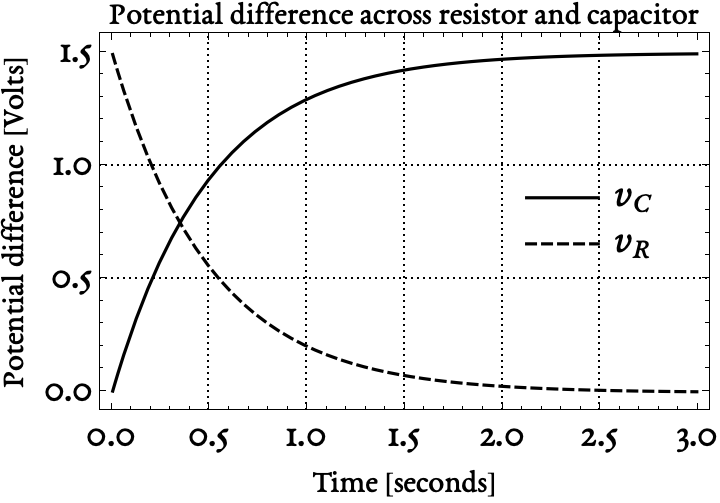
These curves are given by \[ \begin{aligned} v_C(t) &= \frac{3}{2}-\frac{3}{2} e^{-2 t} \\ v_R(t) &= \frac{3}{2} e^{-2 t} \end{aligned} \]
1.2 Power dissipation
The power dissipated by an electrical component equals the voltage across it times the current through it. With this principle in mind, we can write the following equation for the power \(p_R\) dissipated by a resistor.

\[ \begin{aligned} p_R = v_R i_R &= (i_R R) i_R = i_R^2 R \\ &= v_R \left( \frac{v_R}{R} \right) = \frac{v_R^2}{R} \end{aligned} \]
- Write a mathematical expression for the power dissipated by the resistor in Figure 1, assuming that \(v_C(0) = 0\) as before. If you use units correctly, this answer should be in Watts.
- Use this expression to calculate the total amount of energy dissipated by the circuit in its first ten seconds of operation. Give your answer in Joules or multiples of Joules.
- If there was no capacitor in the circuit in Figure 1, how much more energy would be dissipated by the resistor in the first ten seconds of its operation? Divide this number by the answer from (b) to give a ratio.
The power dissipated in the resistor is given by \[ \begin{aligned} p_R = \frac{v_R^2}{R} &= \frac{(3/2 e^{-2t})^2}{1.25 \times 10^6} \\ &= 1.8 \times 10^{-6}e^{-4t} \end{aligned} \]
The total energy dissipated equals the power integrated over time. So we have \[ \int_0^{10} p_R dt = \int 1.8 \times 10^{-6} \int_0^{10} e^{-4t} = 4.5 \times 10^{-7} \]
If there were no capacitor, then the resistor would remain at a constant voltage and current. So over ten seconds, we would have \(v^2/R\) Watts dissipated, where \(v\) is the initial voltage across the resistor, i.e., 1.5 volts. So we would have \[ \int_0^{10} \left( \frac{1.5^2}{1.25 \times 10^{6}} \right) dt = \left( \frac{1.5^2}{1.25} \right) \times 10^{6} \times 10 = 1.8 \times 10^{-5} \] Joules of energy dissipated. The ratio in question is \[\frac{1.8 \times 10^{-5}}{4.5 \times 10^{-7}} = 40\]
So, forty times less energy is dissipated in the circuit when there is a capacitor than when there is no capacitor.
2 Deriving the equations for a first-order circuit
2.1 Two capacitors in series
Consider the circuit shown below.

Using Kirchhoff’s Laws, derive a differential equation for \(v_2\) and a differential equation for \(v_1\).
State whether the equations are coupled or uncoupled, and linear or nonlinear.
To solve this problem, we first label some nodes as follows.
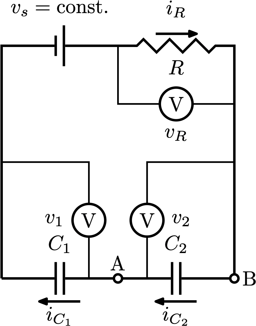
Then, we write Kirchhoff’s current law for node B: \[i_{C_2} - i_{R} = 0 \implies i_{C_2} = i_{R}.\] By the definitions of voltage-current relations for a capacitor and a resistor, this gives us the following equation. \[C_2 \frac{d v_2}{dt} = \frac{V_R}{R}.\]
Then, we write down Kircchoff’s Voltage law for a loop around the circuit to say \[v_s - v_1 - v_2 - v_R = 0 \implies v_R = v_s - (v_1 + v_2).\] Thus, one of the required equations is \[ C_2 \frac{d v_2}{dt} = \frac{v_s}{R} - \frac{(v_1 + v_2)}{R}. \tag{1}\]
We then write Kirchhoff’s current law at node A. This gives \[i_{C_1} - i_{C_2} = 0 \implies i_{C_2} = i_{C_1},\] which can be written in terms of voltages as \[C_1 \frac{d v_1}{dt} = C_2 \frac{d v_2}{dt}. \tag{2}\]
Thus, the two differential equations are
\[ \boxed{ \begin{aligned} R C_2 \dot{v}_2 &= {v_s} - {(v_1 + v_2)} \\ R C_1 \dot{v}_1 &= {v_s} - {(v_1 + v_2)} \end{aligned} } \]
2.2 Two resistors in series
Consider the circuit below.

For this circuit, write down mathematical expressions for the voltage across the resistors and across the capacitor as functions of time.
Also plot these expressions on the same set of axes up to \(t=20\) seconds.
To solve this problem, we first label some nodes as follows.
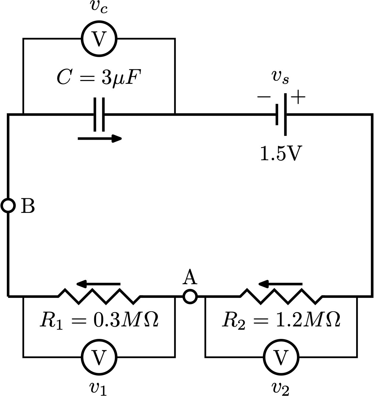
First, write down Kirchhoff’s Voltage Law for a loop around the circuit. We get \[v_s - v_1 - v_2 - v_c = 0. \tag{3}\] Then, we use the current law at node A to say that \[i_{R_1} = i _{R_2} \implies \frac{v_1}{R_1} = \frac{v_2}{R_2}. \tag{4}\] We can then re-write Equation 3 in terms of \(v_2\) and eliminate \(v_1\): \[v_s - v_1 - v_1 \frac{R_2}{R_1} - v_c = 0 \implies v_s - v_1 \left( 1+ \frac{R_2}{R_1}\right) - v_c = 0.\] Next, we apply Kirchhoff’s Current Law at node B to write \[i_{R_2} = i_C \implies \frac{v_2}{R_2} = C \frac{d v_c}{dt}. \tag{5}\] But since this current is also equal to the current in and out of node A, we have \[\frac{v_1}{R_1} = C \frac{d v_c}{dt}\] as well. We are now ready to re-write Equation 3 in terms of just one unknown quantity, \(v_c\). Let’s substitute the previous equation into Equation 3 to get \[ \begin{aligned} v_s - v_1 \left( 1 + \frac{R_1}{R_1} \right) - v_c &= 0 \\ v_s - \dot{v}_c R_1 C \left( 1 + \frac{R_1}{R_1} \right) - v_c &= 0 \\ \dot{v}_c R_1 C \left( 1 + \frac{R_2}{R_1} \right) + v_c &= v_s \end{aligned} \]
At this point, it seems like a good idea to expand and simplify the terms. We can write \[R_1 C \left( 1 + \frac{R_2}{R_1} \right) = R_1 C \left( \frac{R_1 + R_2}{R_1} \right) = C(R_1 + R_2).\] Using the symbol \(R_T \equiv R_1 + R_2\) to refer to the total resistance, we can write a familiar differential equation, \[R_T C \dot{v}_C + v_c = v_s.\]
The next task is to solve this differential equation. Using \(v\) for the unknown variable \(v_c\) and \(\tau \equiv R_T C\) for simplicity, and recalling that \(v_s\) is a constant number that we’ll leave in symbolic form, we have
\[ \begin{aligned} \tau \frac{dv}{dt} + v &= v_s \\ \frac{dv}{v_s-v} &= \frac{dt}{\tau} \\ \int \frac{dv}{v_s-v} &= \int \frac{dt}{\tau} \\ -\log (v_s - v) &= t + c \\ v_s-v &= e^c e^{-t/\tau} \implies v = v_s - e^c e^{-t/\tau}. \end{aligned} \] Using the initial condition: \(v=0\) at \(t=0\), we can solve for \(e^c\) and find that \[0 = v_s - e^c e^{0} \implies e^c = v_s,\] so that the voltage across the capacitor is \[v_c(t) = v_s \left(1 - e^{-t/\tau} \right)\]
We can then use Equation 4 and Equation 5 to work out expressions for \(v_2\) and \(v_1\). We find that
\[ \begin{aligned} v_1(t) &= R_1 C \dot{v}_c \\ &= R_1 C \frac{v_s}{\tau} e^{-t/\tau} \\ &= R_1 C \frac{v_s}{(R_1 +R_2) C} e^{-t/\tau} \\ &= \frac{R_1}{R_1 +R_2} v_s e^{-t/\tau} \end{aligned} \]
and
\[ \begin{aligned} v_2(t) &= R_2 C \dot{v}_c \\ &= R_2 C \frac{v_s}{\tau} e^{-t/\tau} \\ &= R_2 C \frac{v_s}{(R_1 +R_2) C} e^{-t/\tau} \\ &= \frac{R_2}{R_1 +R_2} v_s e^{-t/\tau} \end{aligned} \]
3 Initial Value Problems and integration
3.1 First order systems with zero or constant input
Solve the following initial value problems by integration. The result should be a function \(x(t)\) in which no unknowns remain.
- \(\dot{x} + 3x = 0, x(0) = 2\)
- \(\dot{x} - 3x = 0, x(0) = 2\)
- \(\dot{x} + 3x - 5 = 0, x(0) = 2\)
What do your answers to 1 and 2 above tell us about the physical implication of a circuit in which the resistance were negative? (This doesn’t actually happen; resistance is by nature positive)
Answer: This would imply that the voltage across a capacitor keeps going up toward infinity, which sounds unphysical and bad.
To solve this initial value problem by integration, we first write out the derivative in full, then ‘separate’ the \(dx\) and \(dt\) terms. \[ \begin{aligned} \dot{x} + 3x &= 0, x(0) = 2 \\ \implies \frac{dx}{dt} + 3x &= 0 \\ \frac{dx}{dt} &= -3x \\ \frac{dx}{x} &= -3dt \\ \int \frac{dx}{x} &= \int -3 dt \\ \log x &= -3t + c \\ e^{\log x} &= e^{-3t+c} \\ x &= e^{c} \cdot e^{-3t} \end{aligned} \] We can then use the initial condition to find the constant of integration, \(c\). \[ 2 = e^{c} e^0 \implies e^c = 2 \implies c = \log 2. \] So the solution to our initial value problem is \[x = 2 \cdot e^{-3t}\]
To solve this initial value problem by integration, we first write out the derivative in full, then ‘separate’ the \(dx\) and \(dt\) terms. \[ \begin{aligned} \dot{x} - 3x &= 0, x(0) = 2 \\ \implies \frac{dx}{dt} - 3x &= 0 \\ \frac{dx}{dt} &= 3x \\ \frac{dx}{x} &= 3dt \\ \int \frac{dx}{x} &= \int 3 dt \\ \log x &= 3t + c \\ e^{\log x} &= e^{3t+c} \\ x &= e^{c} \cdot e^{3t} \end{aligned} \] We can then use the initial condition to find the constant of integration, \(c\). \[ 2 = e^{c} e^0 \implies e^c = 2 \implies c = \log 2. \] So the solution to our initial value problem is \[x = 2 \cdot e^{3t}\]
To solve this initial value problem by integration, we first write out the derivative in full, then ‘separate’ the \(dx\) and \(dt\) terms. \[ \begin{aligned} \dot{x} + 3x - 5 &= 0, \quad x(0) = 2 \\ \implies \frac{dx}{dt} &= 5- 3x \\ \frac{dx}{5-3x} &= dt \\ \int \frac{dx}{5-3x} &= \int dt \\ \frac{1}{-3} \log (5-3x) &= t + c \\ \log (5-3x) &= -3t + c, \quad \text{ redefining } c \\ e^{\log (5-3x)} &= e^{-3t + c} \\ 5 - 3x &= e^c \cdot e^{-3t} \\ \end{aligned} \] We can then use the initial condition to find the constant of integration, \(c\). \[ 5 - 3 \cdot 2 = e^{c} \cdot e^0 \implies e^c = -1 \] So we can substitute this into our expression \[ \begin{aligned} 5 - 3x &= - e^{-3t} \\ x(t) &= \frac{5}{3} + \frac{1}{3} e^{-3t} \end{aligned} \]
3.2 First order systems with ramp input
By multiplying an ‘integrating factor’ of \(e^{2t}\) to both sides of the following equation, solve for \(x(t)\) in the following initial value problem. Give your answer as a mathematical expression in terms of \(t\).
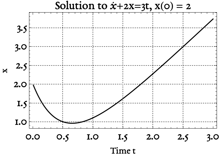
\[\dot{x} + 2x = 3t, x(0) = 2\]
Your function, when plotted against time, should look like the plot below.
First, we write the derivative out explicitly.
\[\frac{dx}{dt} + 2x = 3t\]
Then, we multiply both sides by \(\mu = e^{2t}\)
\[ \mu \frac{dx}{dt} + 2 \mu x = 3 \mu t\]
which is
\[ e^{2t} \frac{dx}{dt} + 2 e^{2t} x = 3 e^{2t} t\]
Recognizing that \(\frac{d}{dt}\) of \(e^{2t}\) is \(2e^{2t}\), we can identify a product rule on the left hand side:
\[ \begin{aligned} \underbrace{e^{2t}}_{\mu} \frac{dx}{dt} + \underbrace{2 e^{2t}}_{\dot{\mu}} x &= 3t e^{2t} \\ \implies \frac{d}{dt} \left( \mu x \right) &= 3te^{2t} \\ \int d \left( \mu x \right) &= \int 3te^{2t}dt \\ \mu x &= \int 3te^{2t}dt \end{aligned} \]
Using integration by parts, we find that the right hand side simplifies to
\[ \begin{aligned} \int 3te^{2t}dt &= \frac{3}{2} t e^{2t} - \int \frac{3}{2} e^{2t} dt \\ &= \frac{3}{2} t e^{2t} - \frac{3}{4} e^{2t} + c \end{aligned} \]
So we can now write
\[ \begin{aligned} \mu x &= \frac{3}{2} t e^{2t} - \frac{3}{4} e^{2t} + c \\ e^{2t} x &= \frac{3}{2} t e^{2t} - \frac{3}{4} e^{2t} + c \\ \implies x &= \frac{3}{2}t e^{2t} e^{-2t} - \frac{3}{4} e^{2t}e^{-2t} + c e^{-2t} \\ &= \frac{3}{2}t - \frac{3}{4} + c e^{-2t}. \end{aligned} \]
The value of \(c\) can be found from the initial condition, i.e.,
\[ \begin{aligned} 2 &= \frac{3}{2} (0) - \frac{3}{4} + c e^{0} \implies c = \frac{11}{4} \end{aligned} \]
so the final result is \[x(t) = \frac{11}{4} e^{-2t} + \frac{3}{2}t - \frac{3}{4}\]
4 Transient and steady-state response
The ‘steady state’ is the behavior that a system displays at large times.
- What is the steady-state voltage across each of the two resistors below respectively?

\(V_{R_1} = 0.3V\) and \(V_{R_2} = 1.2V\)
- What is the steady-state voltage across the two resistors and across the capacitor respectively? For this, you should be able to use your answer from earlier.

\(V_{R_1} = 0\), \(V_{R_2} = 0\), and \(V_{C} = 1.5V\)
- In class, we saw that the response of a first-order system to a ‘ramp input’ looks like a curve followed by a straight line. For the system \[\dot{x} + a x = f(t)\] subjected to a ramp input of the form \(f(t) = c t\), is the slope of the steady-state response equal to the slope of the input?
The expression for the voltage in the ramp circuit shown in We saw, in Section 3.2, that for a system with governing equation \[ \dot{x} + 2x = 3t, \tag{6}\] the voltage as a function of time is \[11/4 \exp(-2 t) + 3/2 t - 3/4.\] At long times, the exponential will just be zero, so the expression will be \[3t/2 -3/4,\] which has a slope of \(3/2\). It appears that, if we cast Equation 6 in the form \[\frac{1}{2} \dot{x} + x = \frac{3}{2}t,\] then the slope of the right-hand side is, again, \(3/2\).
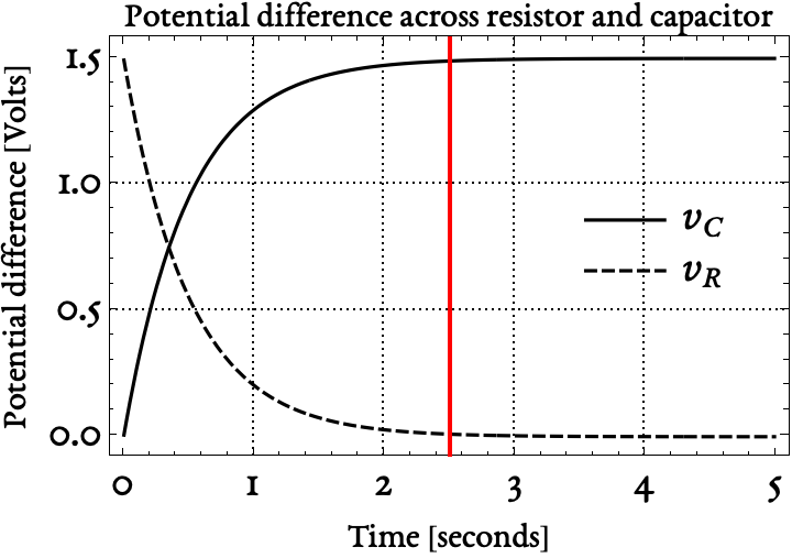
- Make another copy of the figure you made for Section 1.1. On this version of your figure, draw a vertical line representing the time at which the system can be said to have reached steady state. Use the convention discussed in lecture 4, which states that transients die out when \(t = 5\tau\).
We have to make a graph with \(t = 5\tau\) labeled. \(\tau\) for the problem in Section 1.1 is \(\tau = RC = 1/2,\) so \(\tau = 1/2\) and \(5\tau\) is \(2.5\). The required graph looks like
5 Numerical Solution of Initial Value Problems
This is an extension of the in-class activity on Thursday.
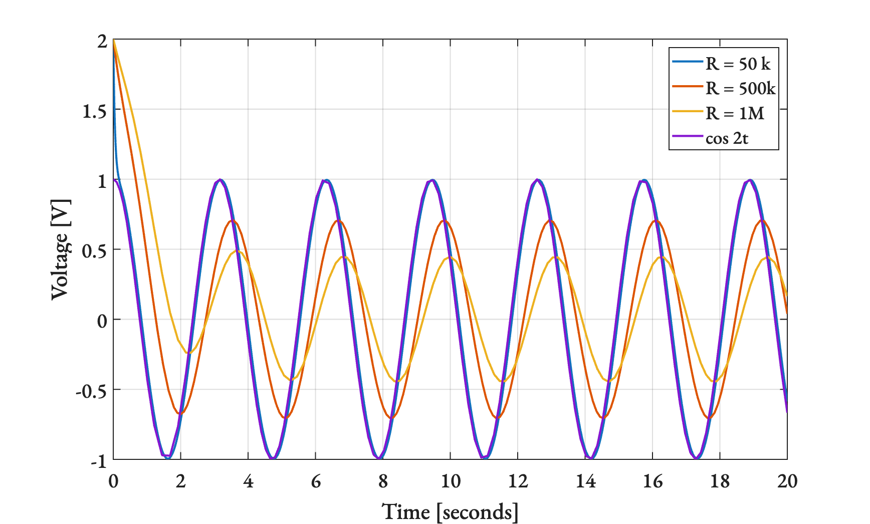
Use ode45 or solve_ivp or NDSolve to determine the voltage across the capacitor from \(t=0\) to \(t=20\). Plot the results on a single set of axes for three values of \(R= \{ 50, 500, 1000 \} k\Omega\). In all cases, assume that the capacitor starts out with a voltage of \(+2\) volts across it. On the same set of axes, also plot \(v_s(t)\), which is given in the problem.

% Define the three tau's
% Three functions for right-hand side.
function dxdt = rhs1(t,x)
    tau1 = 50e3 * 1e-6;
    dxdt = (cos(2*t) - x)/tau1;
end

function dxdt = rhs2(t,x)
    tau2 = 500e3 * 1e-6;
    dxdt = (cos(2*t) - x)/tau2;
end

function dxdt = rhs3(t,x)
    tau3 = 1000e3 * 1e-6;
    dxdt = (cos(2*t) - x)/tau3;
end

% Use ode45 three times with tspan = [0,20], x0 = 2
[t1,x1] = ode45(@rhs1,[0,20],2);
[t2,x2] = ode45(@rhs2,[0,20],2);
[t3,x3] = ode45(@rhs3,[0,20],2);

% Format plot nicely
set(0, 'DefaultLineLineWidth', 2);
plot(t1,x1,t2,x2,t3,x3,t3,cos(2*t3))
legend("R = 50 k","R = 500k","R = 1M","cos 2t")
set(gca,"FontSize",20)
set(gca,"FontName","EB Garamond")
set(gca,"LineWidth",1)
xlabel("Time [seconds]")
ylabel("Voltage [V]")
grid on;

% Save it
saveas(gcf,"MATLABfig.png")