Lecture 13
E12 Linear Physical Systems Analysis
Second-order systems with damping
We now turn our attention to systems of the form
\[m \ddot{x} + b \dot{x} + k x = f(t)\] 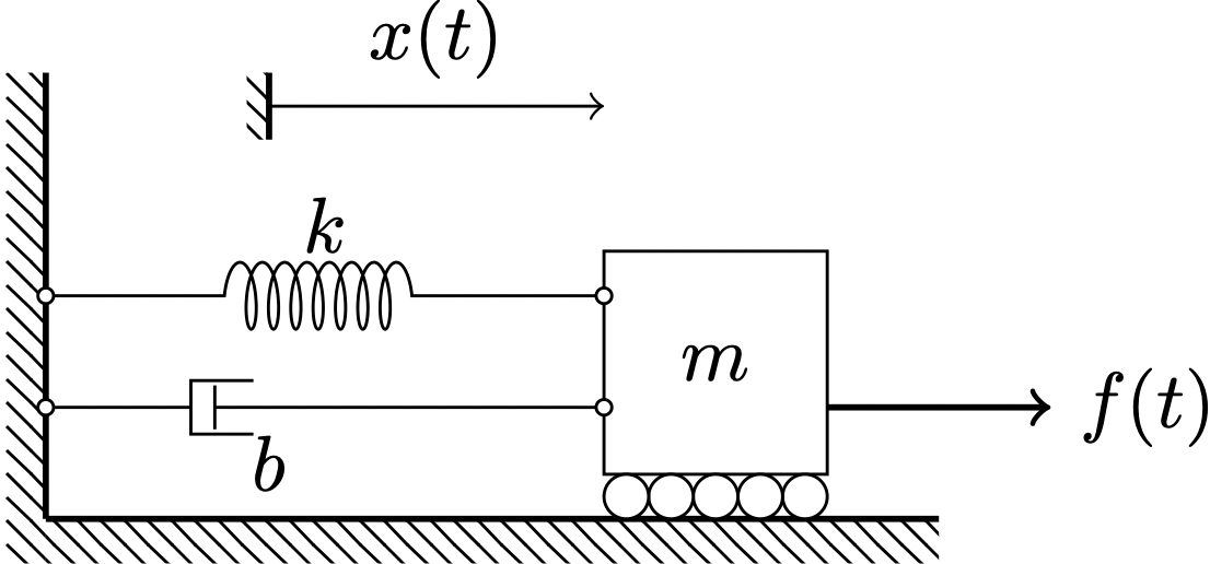
A second-order differential equation for \(x\), the position of the mass
\[L \ddot{q} + R \dot{q} + \frac{1}{C} q = v_{\text{in}}(t)\] 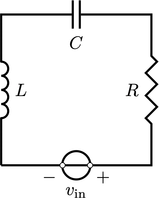
A second-order differential equation for \(q\), the charge on the capacitor
Mass, damping coefficient, spring constant, capacitance, resistance, and inductance are all typically positive
General solution for a second-order differential equation
To solve the equation \[m \ddot{x} + b \dot{x} + k x = f(t), \tag{1}\] let’s start with the ‘free response’ when \(f(t) = 0\).
\[\ddot{x} + a \dot{x} + b x = 0 \tag{2}\]
- Guess a solution: Let’s try \(x(t) = e^{st}\):
- Derivatives are straightforward, and we get \[s^2 e^{st} + a s e^{st} + b e^{st} = 0\] \[(s^2 + as + b )e^{st} = 0\]
- For this to be zero for all \(t\), \(\boxed{s^2 + as + b = 0},\) a.k.a. the characteristic equation for system Equation 2
- Note that \(s^2 + as + b\) is called the characteristic polynomial of Equation 2.
The characteristic equation and its solution
We’ve learned that \(x(t) = e^{st}\) is a solution of \[\ddot{x} + a \dot{x} + b x = 0\] as long as \[s^2 + as + b = 0 \tag{3}\]
- Not just any \(s\) will work.
- \(s\) must solve the quadratic Equation 3.
- Seems like there are two possible values of \(s\) \[s_{1,2} = \frac{-a \pm \sqrt{a^2 - 4b}}{2}\]
Sum of two solutions
We’ve learned that \(x(t) = e^{st}\) is a solution of \[\ddot{x} + a \dot{x} + b x = 0\] as long as \[s^2 + as + b = 0\]
By linearity we know that the sum of two solutions is also a solution. Thus, let’s try: \[x(t) = C_1 e^{s_1 t} + C_2 e^{s_2 t}\]
We can then use two initial conditions \(x(0)\) and \(\dot{x}(0)\) to find \(C_1\) and \(C_2\)
Note: There’s an ‘edge case’ for which this won’t work, i.e., when \(s_1 = s_2\)
If \(s_1=s_2\) the two solutions being added are not really independent, and some math wizardry is needed
A spring-mass-damper problem
Calculate \(x(t)\) for the following system. Leave the answer in terms of ‘constants of integration’, which can later be determined using initial conditions.
Start by ‘guessing’ the following solution \[x(t) = C_1 e^{s_1 t} + C_2 e^{s_2 t}\] for the differential equation \[\ddot{x} + a \dot{x} + b x = 0\]
Solution
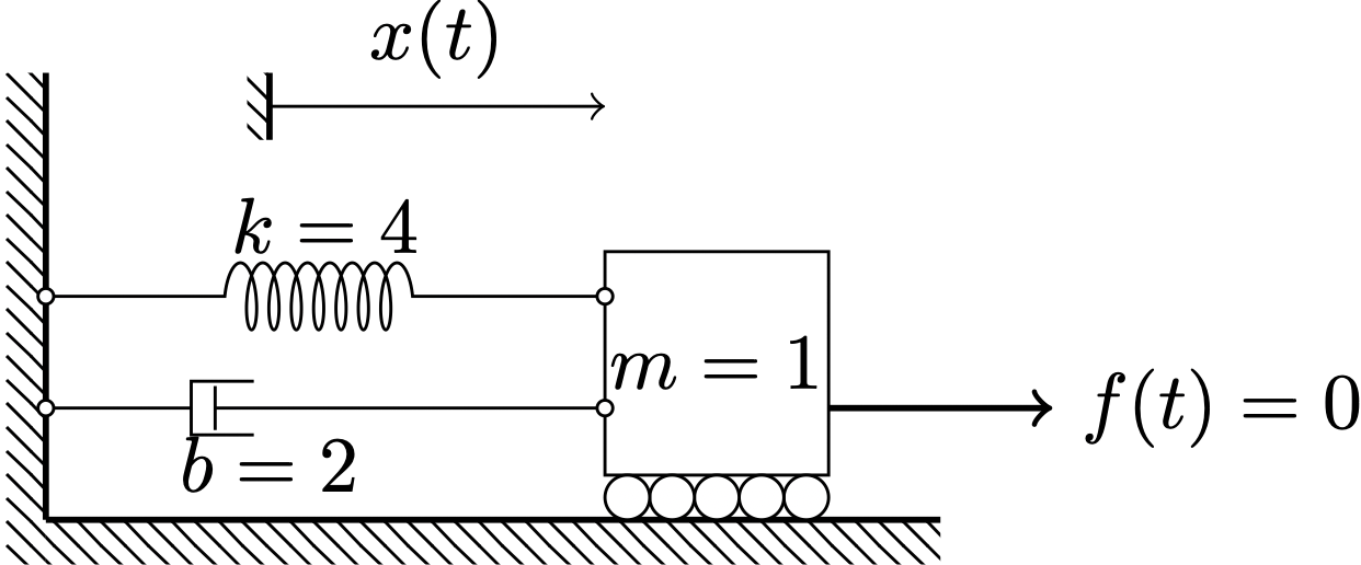
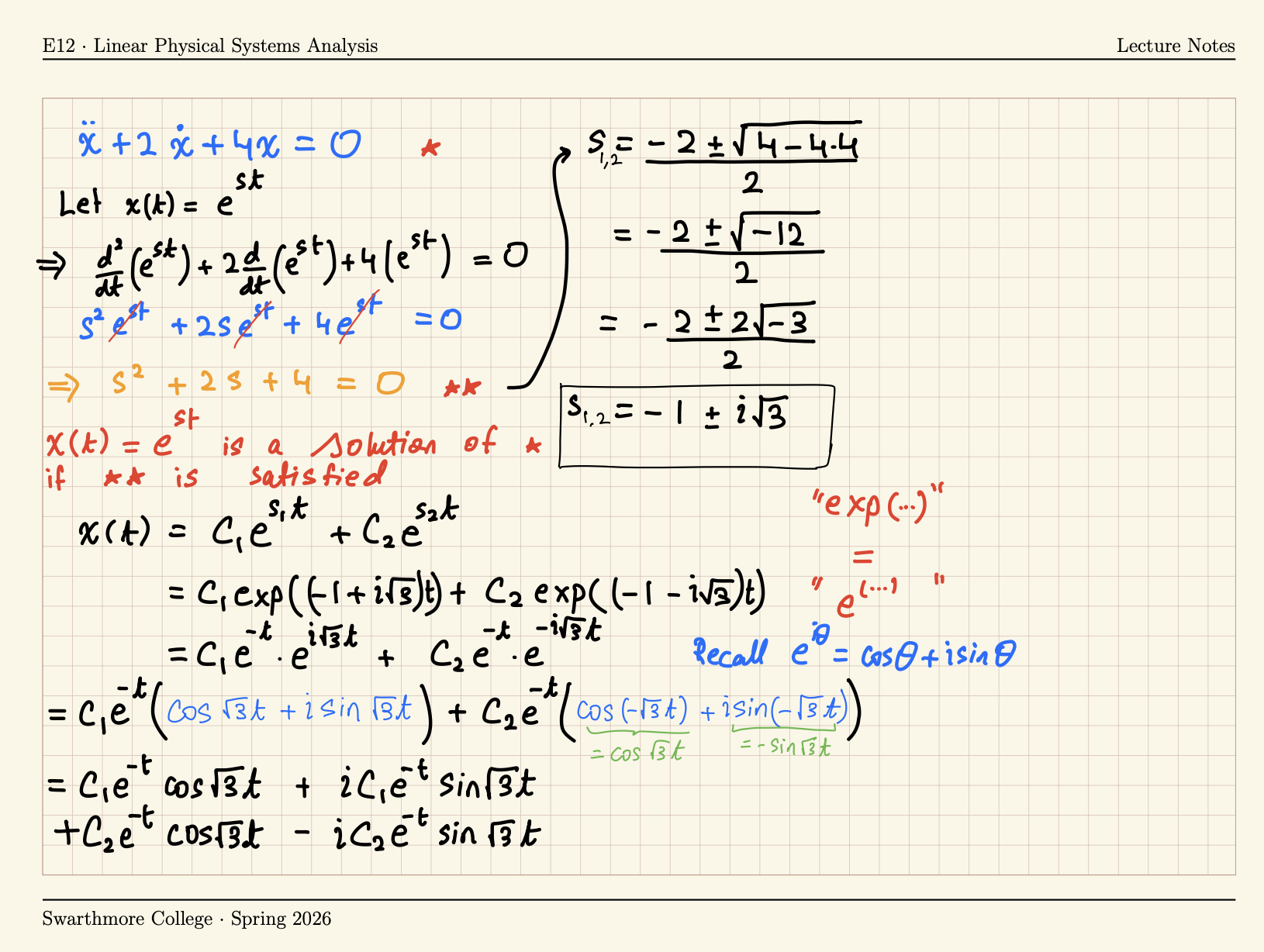
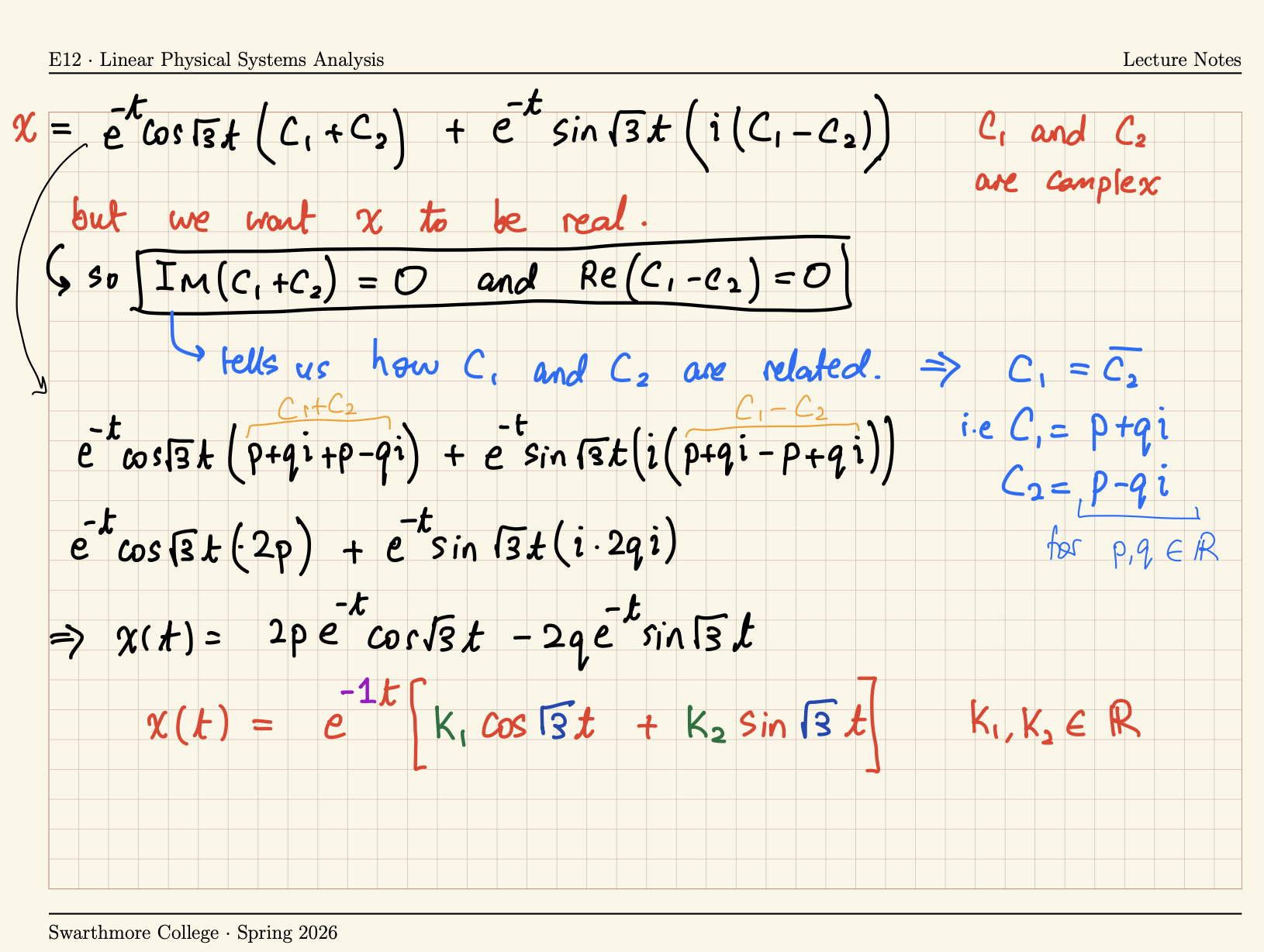
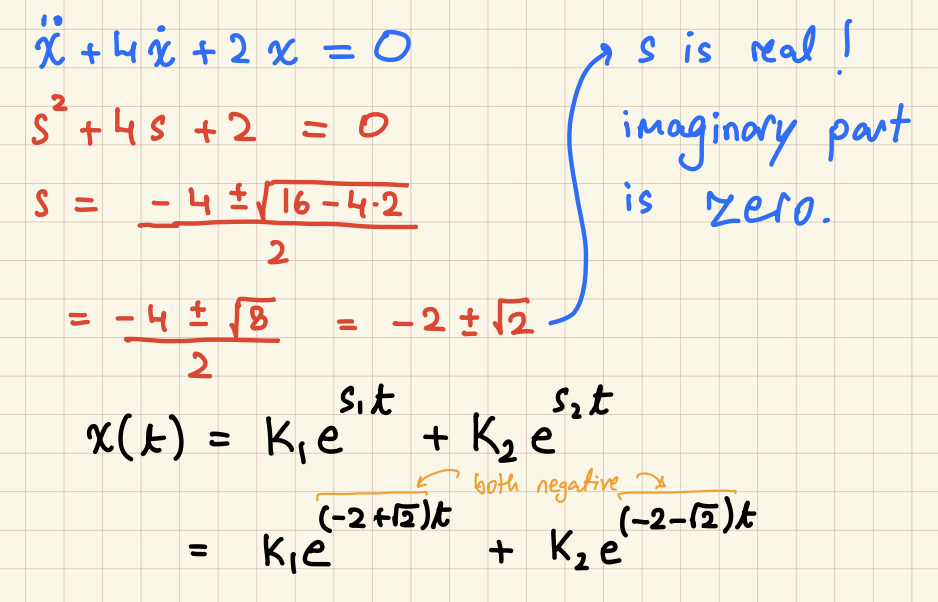
Deriving the solution to \(\ddot{x} + 2 \dot{x} + 4x=0\)
Another spring-mass-damper problem
Calculate \(x(t)\) for the following system. Leave the answer in terms of ‘constants of integration’, which can later be determined using initial conditions.

Start by ‘guessing’ the following solution \[x(t) = C_1 e^{s_1 t} + C_2 e^{s_2 t}\] for the differential equation \[\ddot{x} + a \dot{x} + b x = 0\]
Solution
Effect of increasing damping
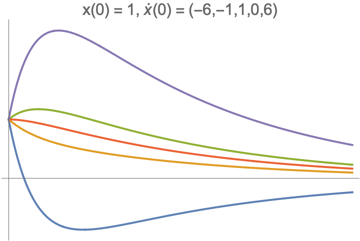
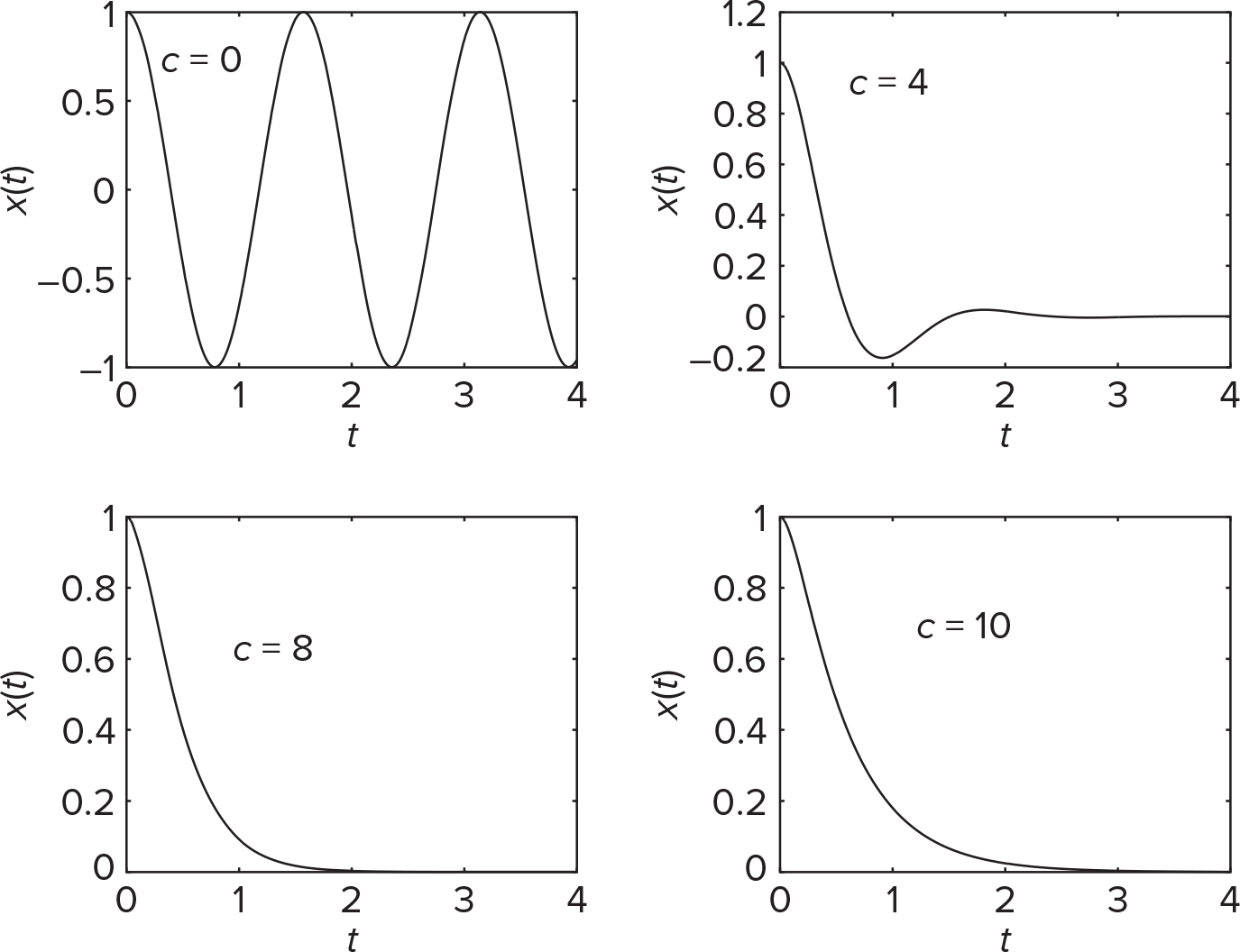
For \(m=1, k = 16\) and \(b = \{ 0, 4, 8, 10\}\), with initial conditions \(x(0) = 1, \dot{x}(0)=0\), let’s look at the free response \(x(t)\) in the absence of any force \(f(t)\).
\[s_{1,2} = \frac{-b \pm \sqrt{b^2-64}}{2}\]
| Damping | Free response \(x(t)\) |
|---|---|
| \(b=0\) | \(x(t) = \cos 4 t\) |
| \(b=4\) | \(x(t) = 1.155 e^{-2t} \sin \left( \sqrt{12} t + 1.047 \right)\) |
| \(b=8\) | \(x(t) = (1+4t) e^{-4t}\) |
| \(b=10\) | \(x(t) = \frac{4}{3} e^{-2t} - \frac{1}{3} e^{-8t}\) |
Procedure for find these:
- Guess a solution \(e^{s t}\)
- Sum two independent solutions \(C_1 e^{s_1 t} + C_2 e^{s_2 t}\)
- \(b=8\) is a special case and has general solution \((C_1 + t C_2)e^{s_1 t}\)
Three Cases
The solutions to \[\ddot{x} + a \dot{x} + b x = 0\] look like \(e^{st}\) where \(s\) depends on the characteristic equation \[s^2 + a s + b = 0, \implies s = \frac{-a \pm \sqrt{a^2-4b}}{2}\]
Depending on the sign of \(\sqrt{a^2 - 4b}\), we have three different cases:
| Case | Roots | Condition | Solution |
|---|---|---|---|
| Case 1 | Two distinct real roots | \(a^2 > 4b\) | \(C_1 e^{s_1t} + C_2 e^{s_2t}\) |
| Case 2 | Two distinct complex roots | \(a^2 < 4b\) | \(e^{rt} \left( C_1 \cos \omega t + C_2 \sin \omega_t \right)\) |
| Case 3 | Repeated real roots (special case) | \(a^2 = 4b\) | \((C_1 + t C_2) e^{s_1 t}\) |
The Roots of a polynomial
Quick recap about polynomials and roots
- A polynomial of degree \(n\) with real coefficients \[f(x) = a_0 x^0 + a_1 x^1 + a_2 x^2 + ... + a_n x^n, \quad a_{1,2,...,n} \in \mathbb{R}\] has \(n\) roots, which we can call \(\lambda_1, \lambda_2, ... \lambda_n\).
- We can factor a polynomial using its roots, so that \[f(x) = (x- \lambda_1)(x-\lambda_2)(x-\lambda_3)...(x-\lambda_n)\]
- The solutions to the equation \(f(x) = 0\) are therefore \(x = \lambda_1, \lambda_2, ..., \lambda_n\)
- The roots of a polynomial with real coefficients need not be real, and in general \(\lambda_{1,2,...,n} \in \mathbb{C}\)
- Any complex roots always show up in conjugate pairs \(\left[ a+bi, a-bi\right]\)
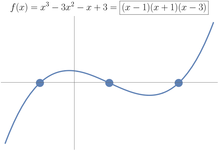
Illustrating roots
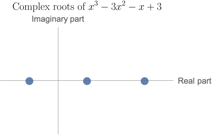
Three roots of a cubic polynomial
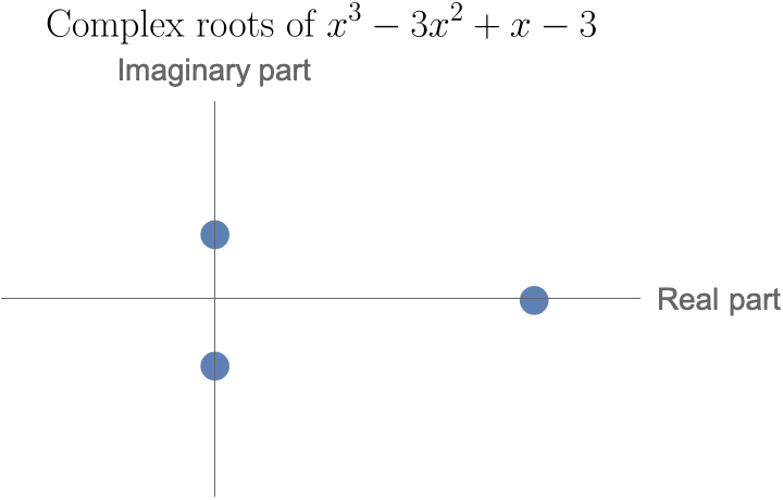
Three One root of a cubic polynomial ?
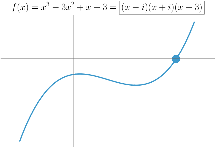
Why does it look like there is only one root?
Illustrating roots on the complex plane instead:
What are the roots of the polynomial \(x^3+3x^2+x-5\) ? Hint: one of the roots is \(x = 1\)
Case 1
When the polynomial \(s^2+as+b\) has real roots, i.e., when solutions to the equation \[s^2+as +b = 0\] are real. Recall that the solution is \(\displaystyle s = \frac{-a \pm \sqrt{a^2-4b}}{2}\).
| Case | Roots | Condition | Solution (example) |
|---|---|---|---|
| Case 1 | Two distinct real roots | \(a^2 > 4b\) | \(x(t) = C_1 e^{s_1t} + C_2 e^{s_2t}\) |
| Case 1a | Both negative | \(a > \sqrt{a^2-4b} > 0\) | |
| Case 1b | One positive one negagtive | \(\sqrt{a^2-4b} > a > 0\) | |
| Case 1c | Both positive | \(\sqrt{a^2-4b} > 0 > a\) | |
| Case 2 | Two distinct complex roots | \(a^2 < 4b\) | \(e^{rt} \left( C_1 \cos \omega t + C_2 \sin \omega_t \right)\) |
| Case 3 | Repeated real roots | \(a^2 = 4b\) | \((C_1 + t C_2) e^{s_1 t}\) |
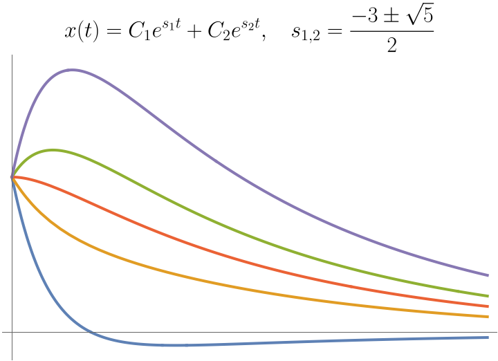
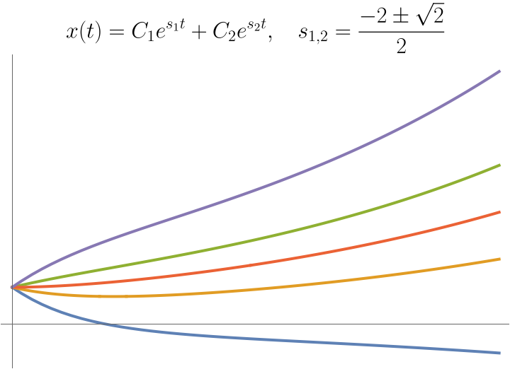
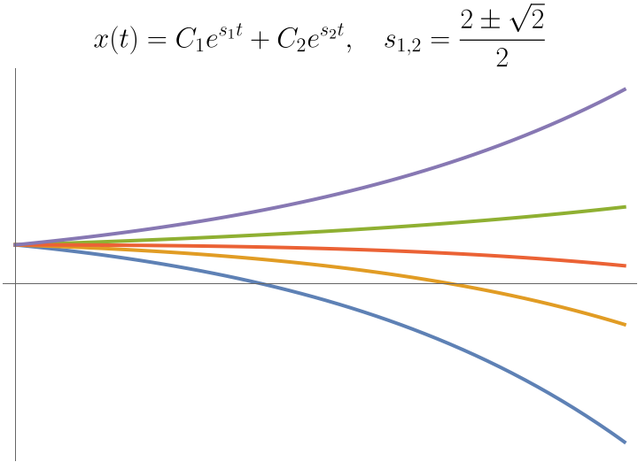
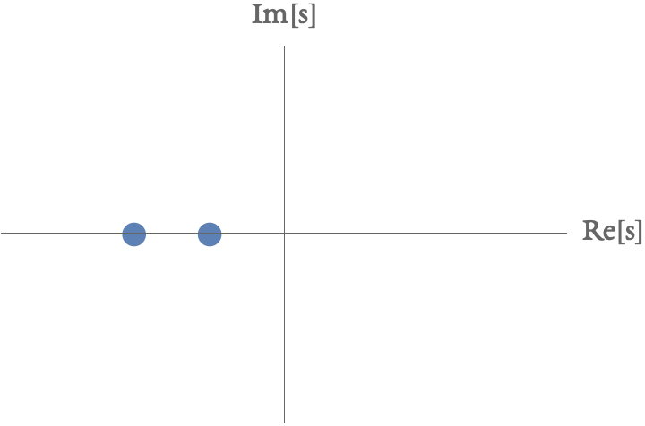
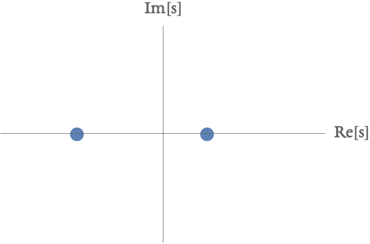
Case 1: Illustrate solutions \(x(t)\) when \(s \in \mathbb{R}\)
| Case 1a: \(s_1,s_2 < 0\) | Case 1b: \(s_1< 0<s_2\) | Case 1c: \(s_1, s_2 > 0\) |
|---|---|---|
| Both roots negative | One positive, one negative | Both roots positive |
 |
 |
 |
 |
 |
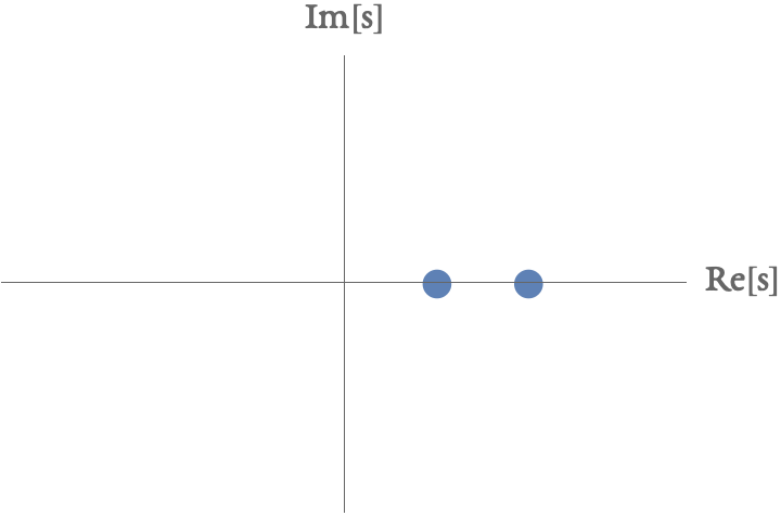 |
Case 2
When the polynomial \(s^2+as+b\) has complex roots, i.e., when solutions to the equation \[s^2+as +b = 0\] are complex.
Recall that the solution is \(\displaystyle s = \frac{-a \pm \sqrt{a^2-4b}}{2}\).
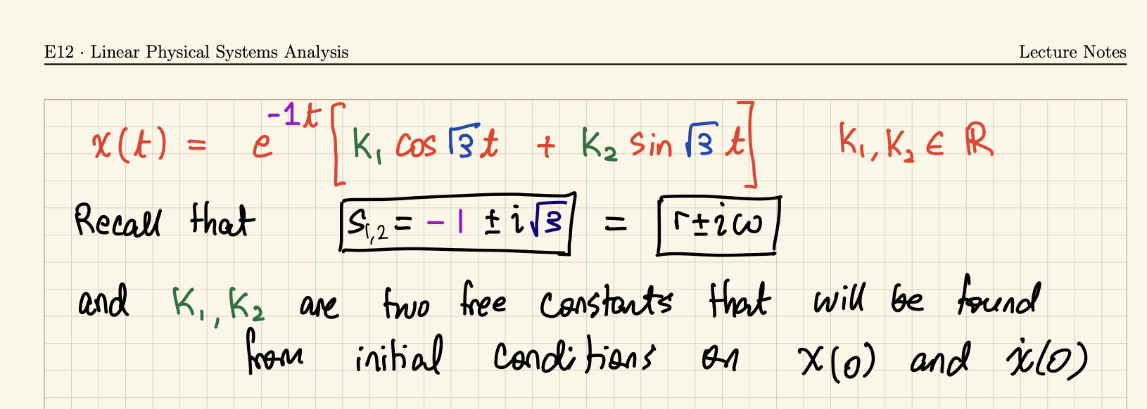
\(s_{1,2} = \frac{-a \pm \sqrt{a^2 - 4b}}{2} = r \pm i \omega\)
| Case | Roots | Condition | Solution (example) |
|---|---|---|---|
| Case 1 | Two distinct real roots | \(a^2 > 4b\) | \(x(t) = C_1 e^{s_1t} + C_2 e^{s_2t}\) |
| Case 2 | Two distinct complex roots | \(a^2 < 4b\) | \(e^{rt} \left( C_1 \cos \omega t + C_2 \sin \omega_t \right)\) |
| Case 2a | Real part negative | \(a < 0\) | |
| Case 2b | Real part positive | \(a > 0\) | |
| Case 2c | Real part zero | \(a = 0\) | |
| Case 3 | Repeated real roots | \(a^2 = 4b\) | \((C_1 + t C_2) e^{s_1 t}\) |
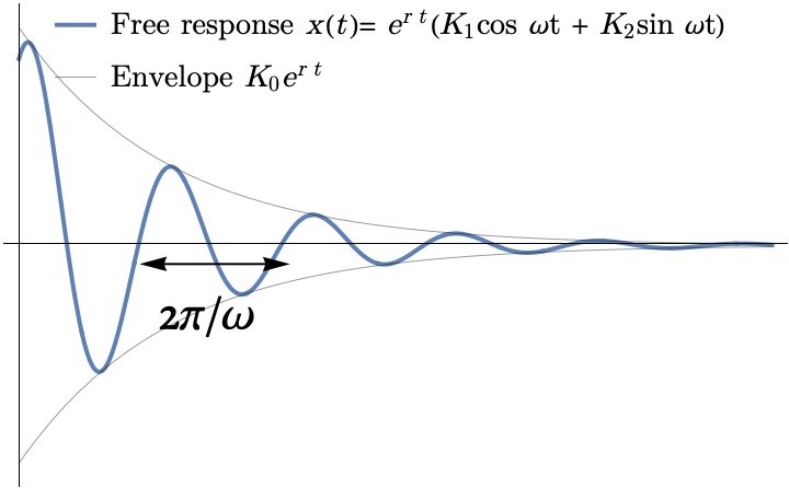
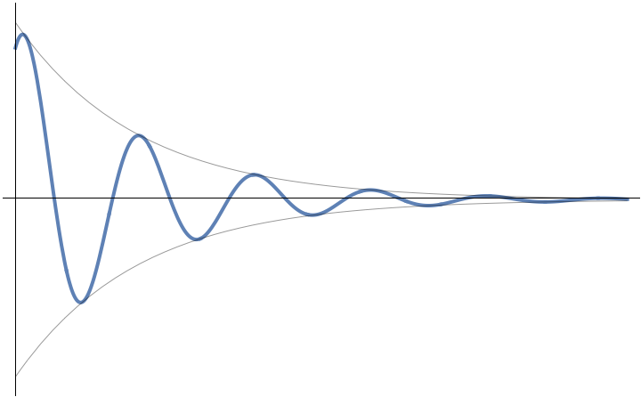
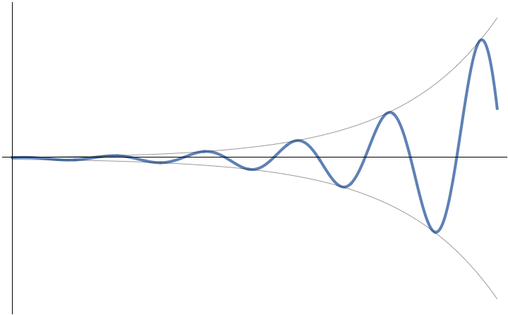
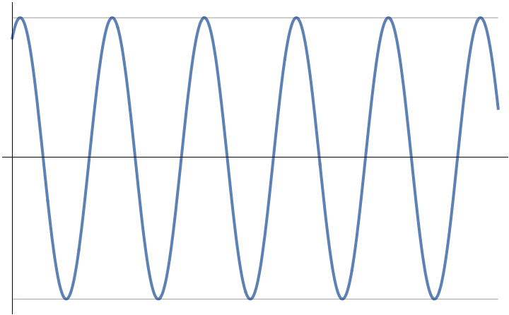
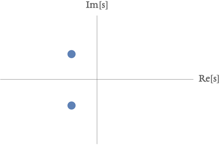
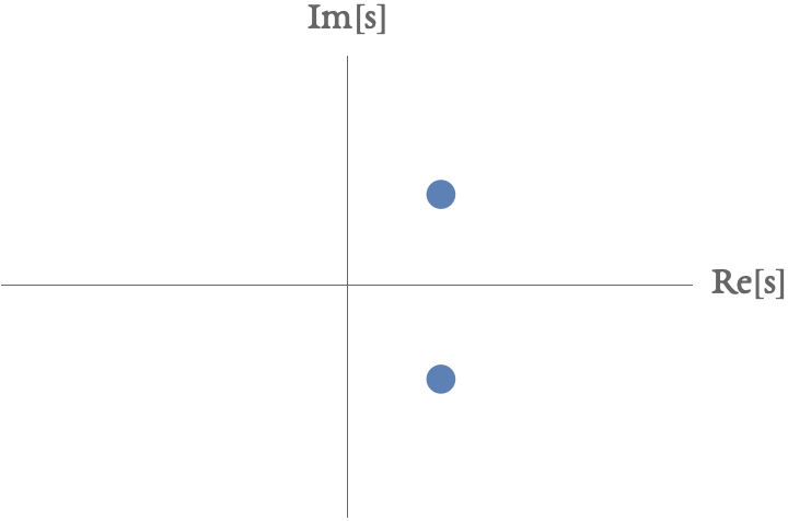
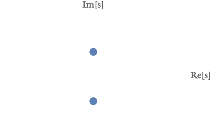
Case 2: Illustrate solutions \(x(t)\) when \(s \in \mathbb{C}\)
| Case 2a: \(r < 0\) | Case 2b: \(r > 0\) | Case 2c: \(r = 0\) |
|---|---|---|
| \(e^{-t} C_0 \cos(\omega t + \phi )\) | \(e^{+t} C_0 \cos(\omega t + \phi )\) | \(e^{0} C_0 \cos(\omega t + \phi )\) |
| \(e^{-t} ( C_1 \cos \omega t + C_2 \sin \omega t\) | \(e^{+t} ( C_1 \cos \omega t + C_2 \sin \omega t\) | \(e^{0} ( C_1 \cos \omega t + C_2 \sin \omega t\) |
 |
 |
 |
 |
 |
 |