Lecture 20

E12 Linear Physical Systems Analysis

The Frequency response

The steady-state output of a linear system with transfer function \(T(s)\), when the input is \[A \sin \omega t,\] is \[B \sin (\omega t + \phi).\] To understand the frequency response of a system, we make use of the complex number \(T(i \omega)\). The magnitude ratio is given by the magnitude of this complex number, \[\frac{B}{A} = \left| T(i \omega) \right|\] and the phase shift is given by the argument of this complex number \[ \phi = \arg T(i \omega)\]

Constructing the bode plot

Find the amplitude ratio of the frequency response for the following functions

1. \[m \dot{v} + b v = f(t)\]
2. \[T(s) = \frac{1}{s+3}\]
3. \[T(s) = \frac{2}{3s+1}\]

\[\frac{B}{A} = \left| T(i \omega) \right|\] \[\phi = \arg T(i \omega)\]

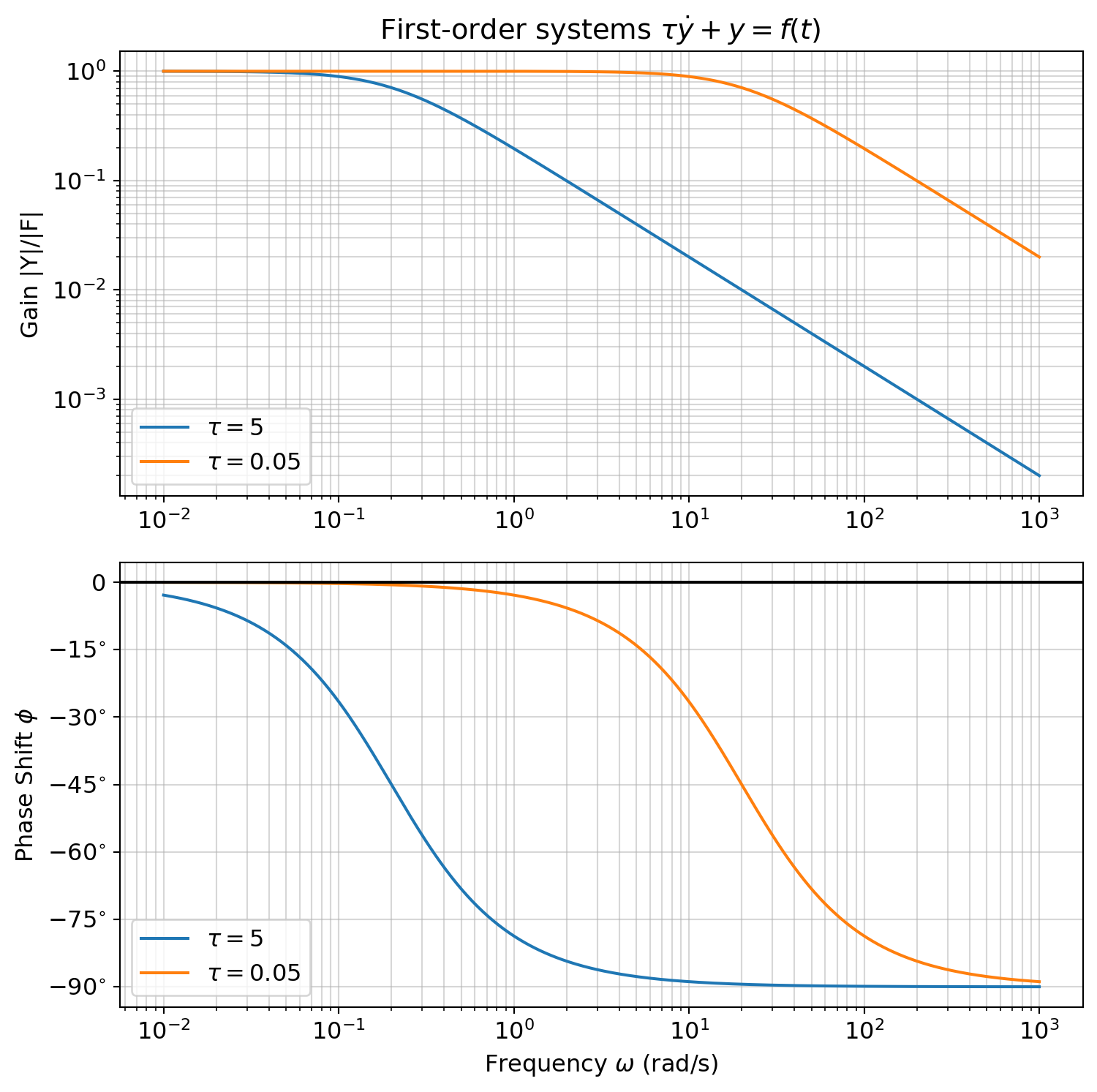
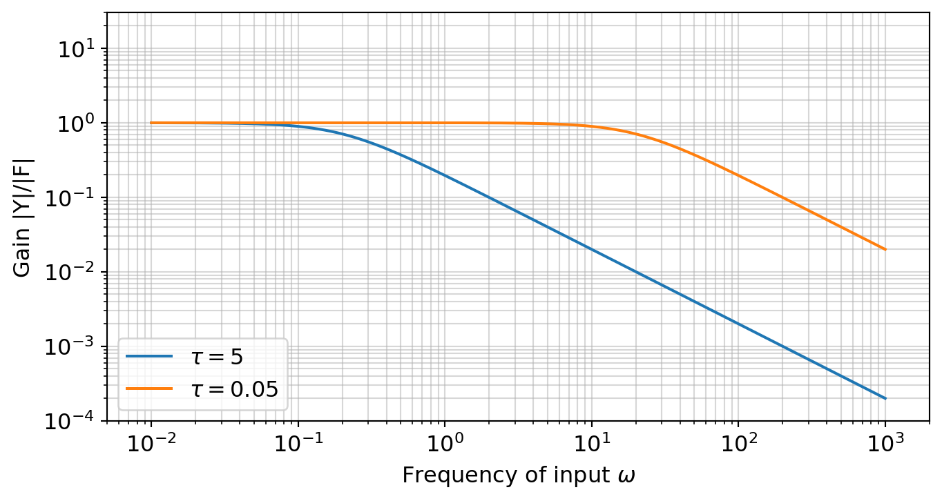
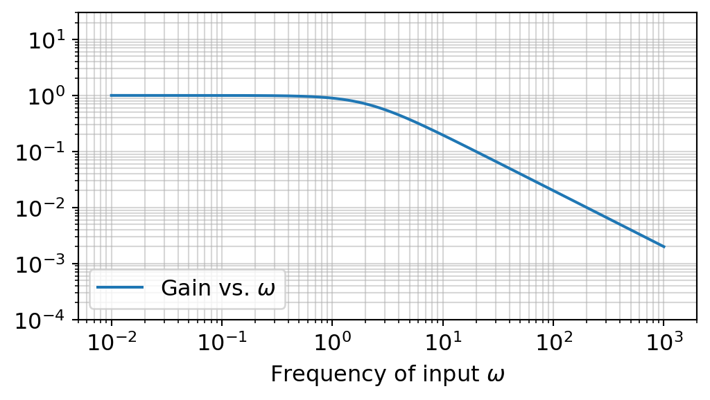
Bode Plots for first-order systems

It is typical to draw Bode plots with a logarithmic scale for the magnitude ratio (a.k.a. gain).

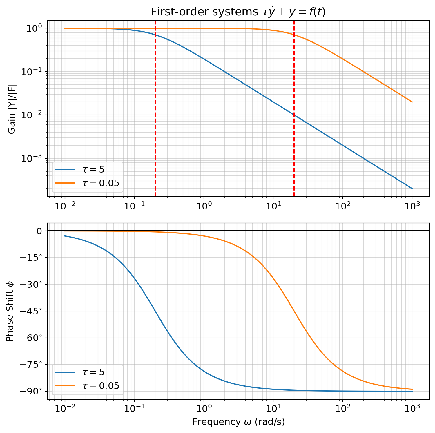
Corner Frequency

The corner frequency of a system refers to the frequency beyond which an applied sinusoidal signal begins to be attenuated by the system.

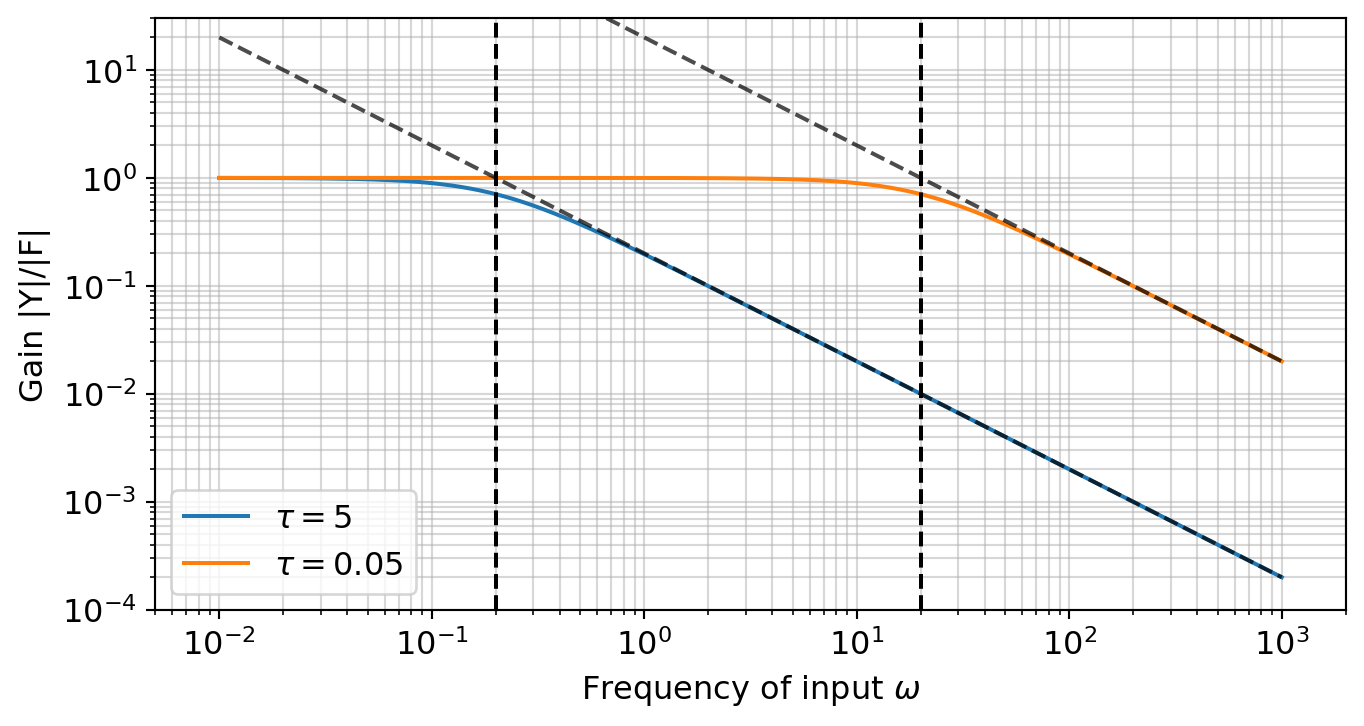
• Beyond the corner frequency, bode plots of first-order systems look like straight line graphs on log-log axes!

Low-frequency and High-frequency approximations

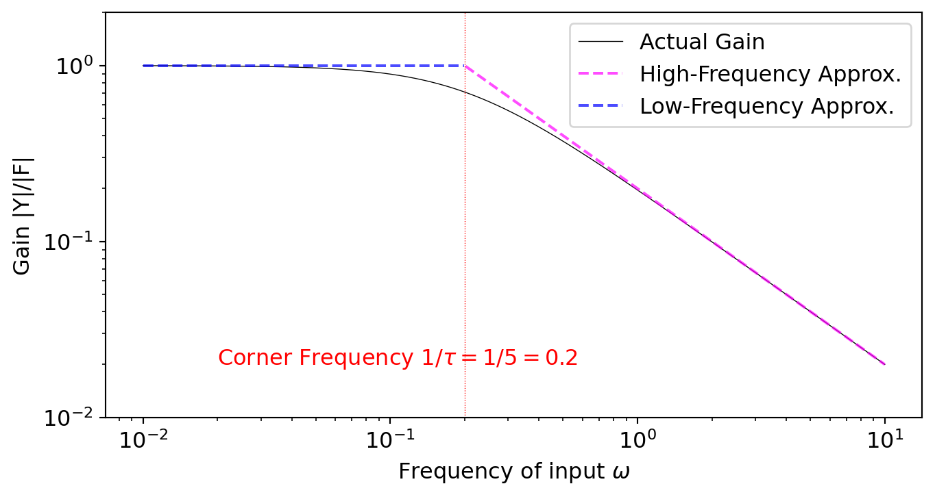
\[T(s) = \frac{1}{\tau s + 1}\]

• At low frequencies \(\omega \ll 1/\tau\), \(\displaystyle |T(i\omega)| = \frac{1}{\sqrt{1+\tau^2\omega^2}} \approx \frac{1}{1}\)
• At high frequencies \(\omega \gg 1/\tau\), \(\displaystyle |T(i \omega)| = \frac{1}{\sqrt{1+\tau^2 \omega^2}} \approx \frac{1}{\sqrt{\tau^2 \omega^2}} = \frac{1}{\tau \omega} = \frac{1}{\tau} \omega^{-1}\)
  • Recall that a straight line on a log-log plot equals a power law on a linear plot, i.e., \[ \begin{aligned} \log y &= k \log x + \log a \\ y &= a x^k \end{aligned} \]
  • Therefore, at high frequencies, the magnitude ratio Bode plot is a straight line with slope = \(-1\)
• At the precise frequency \(\omega = 1/\tau\), we say that the Bode plot has ‘turned the corner’ and therefore the corner frequency equals \(1/\tau\)

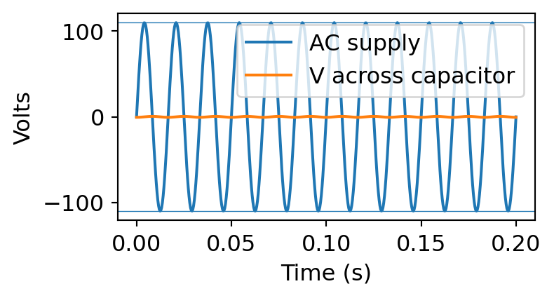
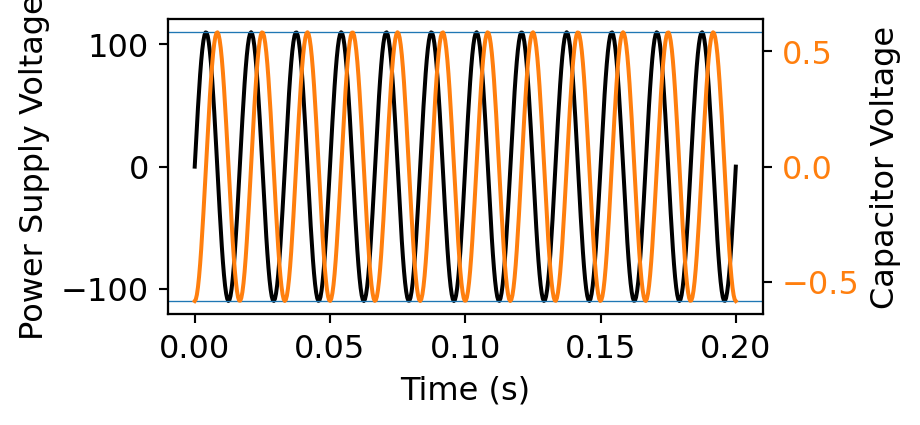
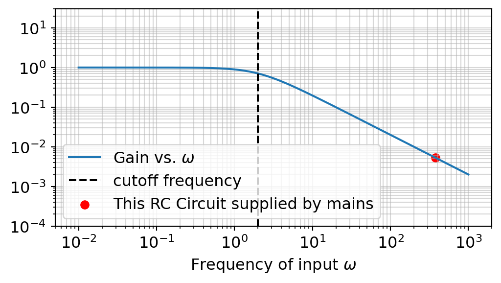
RC Circuit with AC input

Consider an RC circuit with governing equation \[RC \dot{v} + v = v_{\text{in}}(t)\] where \(v_{\text{in}}\) is the usual United States mains power supply, which:

• is at 110 Volts a.c. (alternating current)
• has a frequency of 60 Hertz

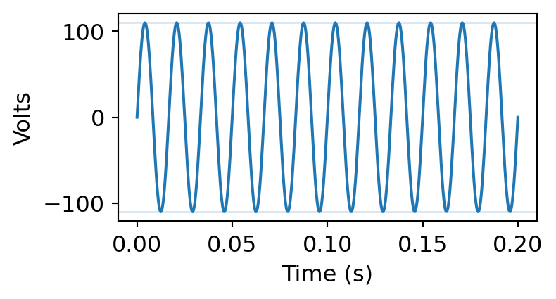
Determine the voltage across the capacitor as a function of time. Recall that \(\omega = 2\pi f\) relates angular frequency to (regular) frequency.

RC Circuit with AC input: solution

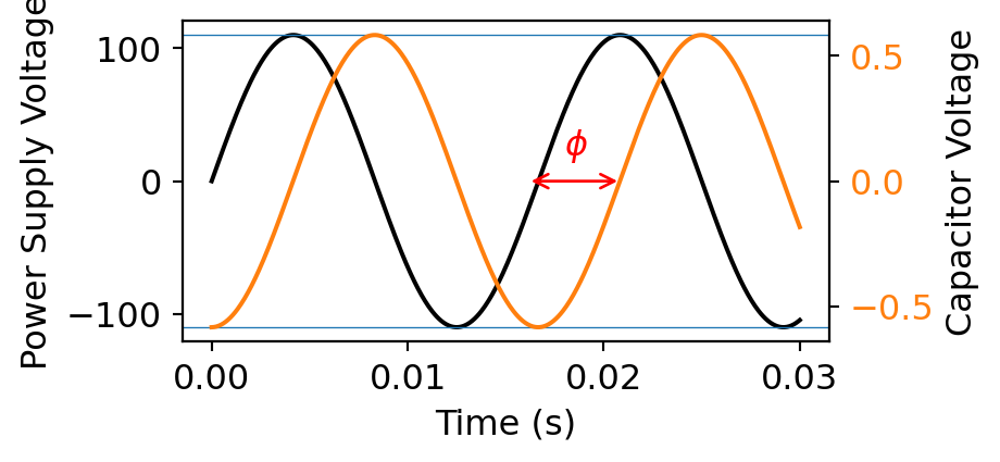
\[ \begin{aligned} T(s) &= \frac{1}{RC s + 1} \\ T(i \omega) &= \frac{1}{i \omega RC + 1} \\ |T(i \omega)| &= \left| \frac{1}{i \omega RC + 1} \right| \\ &= \frac{1}{\sqrt{1+\omega^2(RC)^2}} \\ \arg T(i \omega) &= \tan^{-1}(- \omega \tau) \\ &= \tan^{-1}(- RC \omega) \end{aligned} \]

\[ \begin{aligned} RC &= 1.25 \times 10^{6} \\ & \times 0.4 \times 10^{-6} \\ &= 0.5 \text{ seconds} \\ \omega &= 2 \pi f \\ &= 2 \pi \times 60 \\ &= 120 \pi \text{ rad sec}^{-1} \\ &\approx 377 \end{aligned} \]

Zeros of the Transfer function

• So far, we have been interested in the poles of the Transfer Function, i.e., the roots of the polynomial \(D(s)\) in the fraction \[T(s) = \frac{N(s)}{D(s)}\]
• What about the zeros of the transfer function, i.e., the roots of the polynomial \(N(s)\) ?

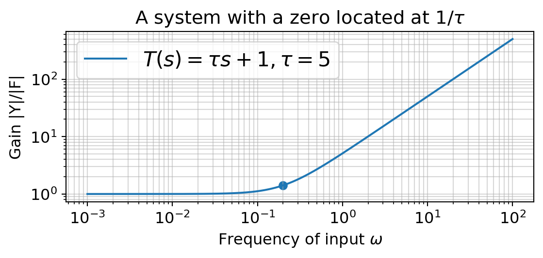
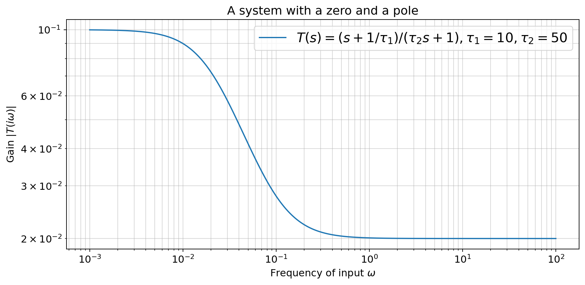
A Zero and a Pole

Generally, we expect a (real) zero to contribute an upward turn and a (real) pole to contribute a downward turn in the Bode plot of a transfer function.

The system shown below has transfer function \[\frac{s+\frac{1}{\tau_1}}{\tau_2 s + 1}\] which has a zero at \(s=-1/\tau_1\) and a pole at \(s = -1/\tau_2\), where \(\tau_1 =10\) and \(\tau_2=50\). Therefore, there is a ‘downward turn’ associated with the pole and an upward pole associated with the zero.

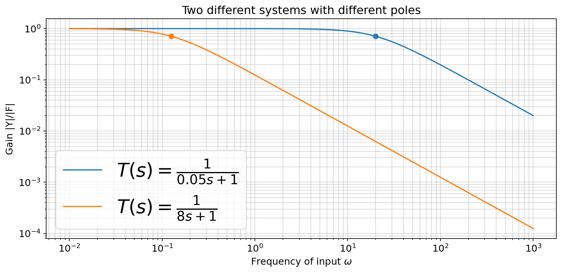
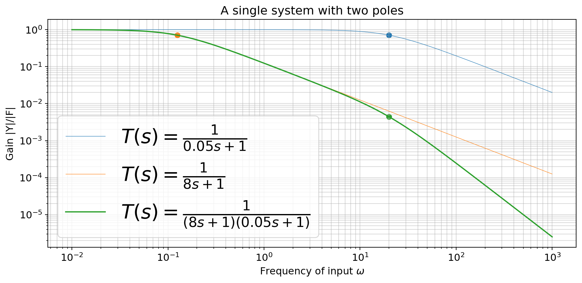
Multiple Poles

What about systems with multiple poles?

Determine the magnitude of \(T(i \omega)\) for the system given by \(T(s)= \displaystyle \frac{1}{(\tau_1 s +1)(\tau_2 s + 1)}\)