Lecture 8

E12 Linear Physical Systems Analysis

The Transfer Function of a system and the Impulse Response of that system

Consider the system \[m \dot{v} + b v = f_a(t)\] where \(v(t)\) is the output and \(f_a(t)\) the input.

Find the transfer function

\[ \begin{aligned} m s V(s) + b V(s) = F_a(s)& \\ V(s) = \frac{1}{ms + b} F_a(s)& \\ \implies \frac{V(s)}{F_a(s)} = \underbrace{\boxed{\frac{1}{m s + b}}}_{\text{Transfer Function}}& \end{aligned} \]

Find \(v(t)\) when \(f_a(t) = \delta (t)\)

\[ \begin{aligned} m s V(s) + b V(s) &= \mathcal{L} \left[ \delta (t) \right] \\ m s V + b V &= 1 \\ \implies V(s) = \underbrace{\boxed{\frac{1}{ms+b}}}_{\text{Impulse Response}} \end{aligned} \]

• The Transfer Function of a system is also the Laplace Transform of that system’s (unit) impulse response.

Block Diagrams

A block diagram is a visual representation of a system, its inputs & outputs, and the relations between the different components.

For example, the block diagram below

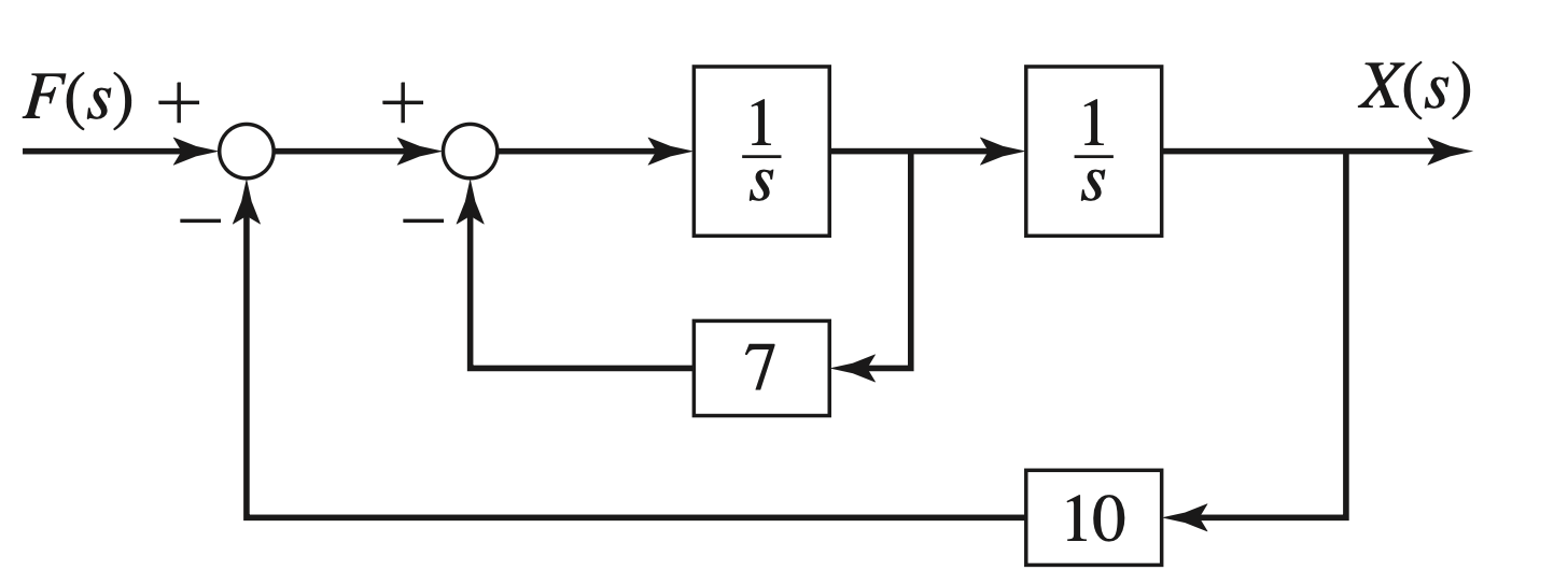
corresponds to the second-order system \[\ddot{x} + 7 \dot{x} + 10x = f(t)\]

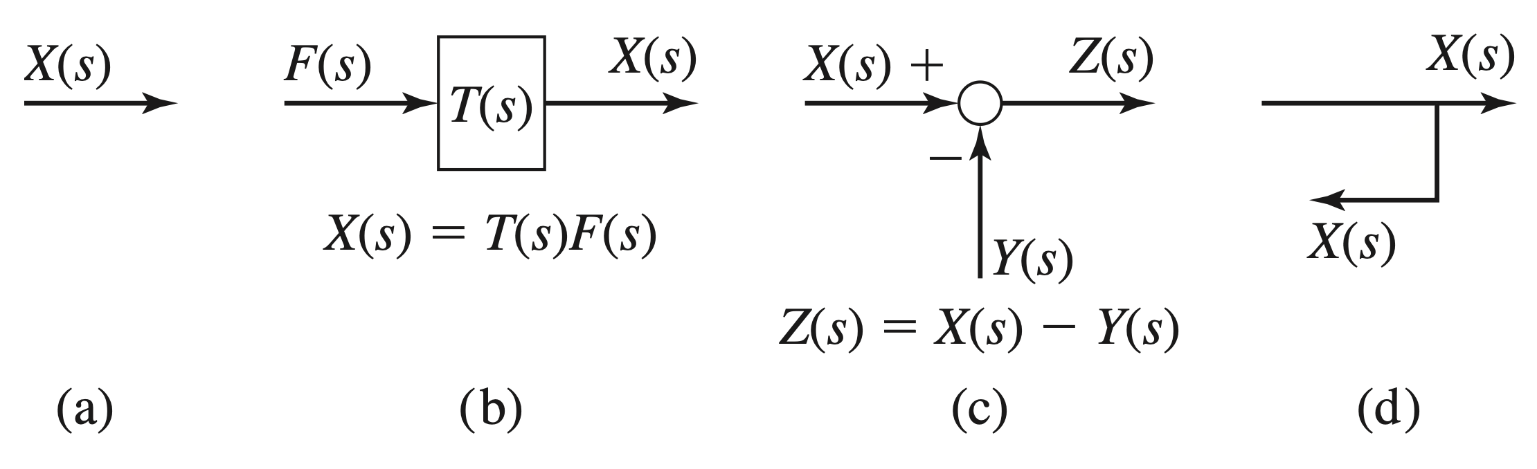
What makes up a block diagram

There are 4 building blocks.

1. The arrow: a variable and the cause-effect relation
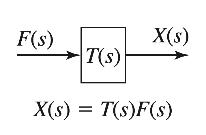
2. The block: a Transfer Function
3. The summer: adds or subtracts
4. The takeoff point: a perfect copy of a variable

Some simple block diagrams

1. Input and output are related algebraically, with no calculus:

This corresponds to the system \(x(t) = K f(t)\)

This corresponds to the system \(x(t) = f(t) + g(t)\)

2. Input and output are related by a differential equation

This corresponds to the system \[ \begin{aligned} \dot{x}(t) &= f(t) \\ \implies sX(s) &= F(s) \\ \implies X(s) &= \frac{1}{s} \times F(s) \end{aligned} \]

Making a simple block diagram

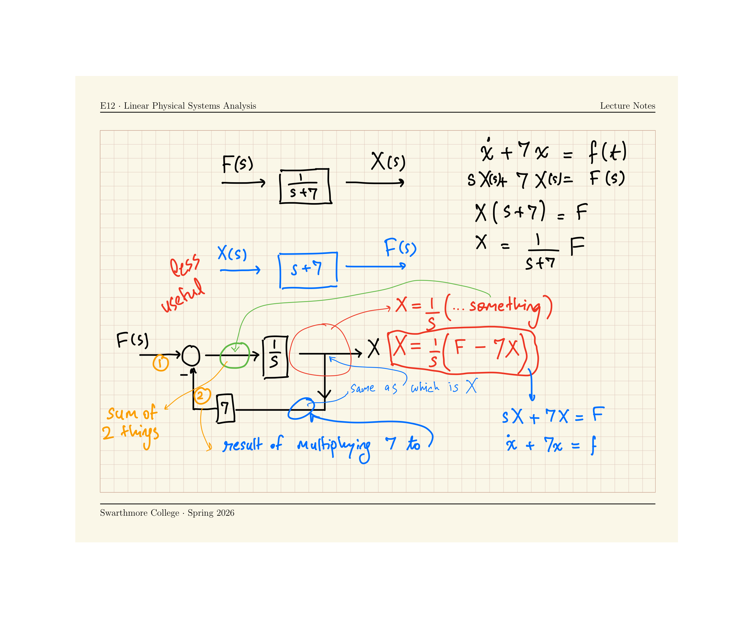
In-class task: Consider the system \(\dot{x} + 7x = f(t)\). Make a block diagram for this system using the shape shown below.

First-order single-input single-output systems

• Block diagram for one input and one output related by a transfer function is

• This is not very useful. But the same system can be drawn in multiple ways! \(\dot{x} + 7 x = f(t)\)

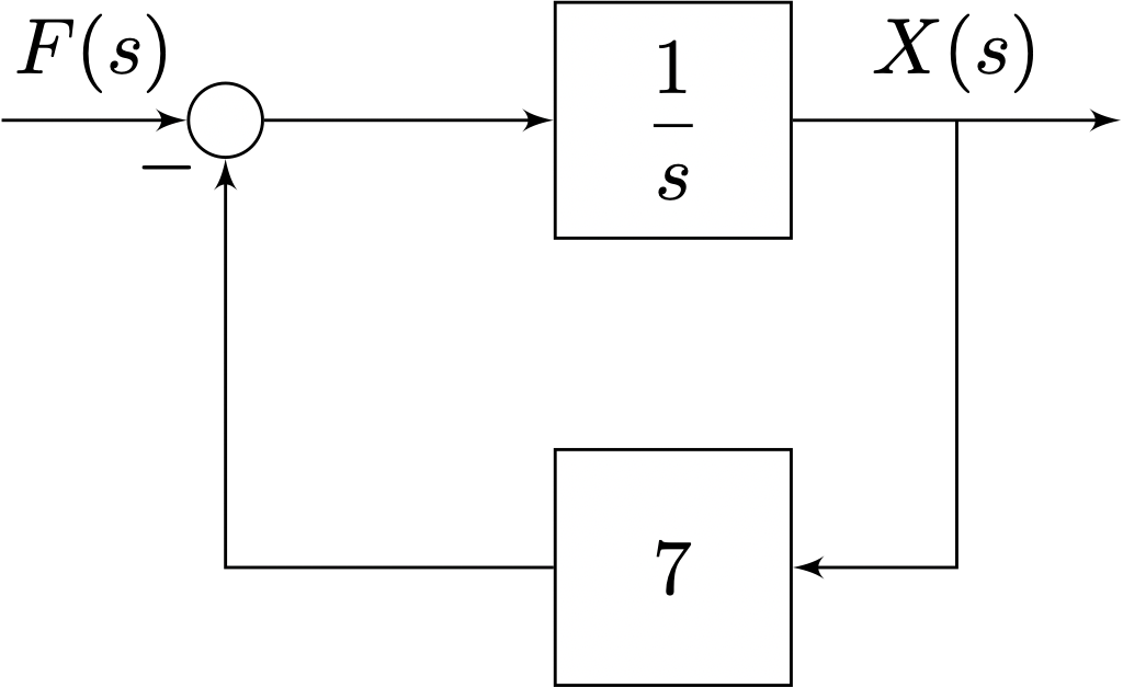\(\displaystyle X(s) = \frac{1}{s} \left( F(s) - 7 X(s) \right)\)

\(\displaystyle X(s) = \frac{1}{s+7} F(s)\)

Anatomy of a block diagram

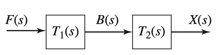
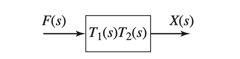
Blocks in series

The following are equivalent

Equivalent block diagrams: the feedback loop

In-class task: Consider the system below. Express \(X(s)\) as a function of \(G(s)\), \(H(s)\) and \(F(s)\). Then put these equations into a simple block diagram where \(X(s)\) and \(F(s)\) are related by a single transfer function.

Hint: Eliminate \(A\) and \(B\).

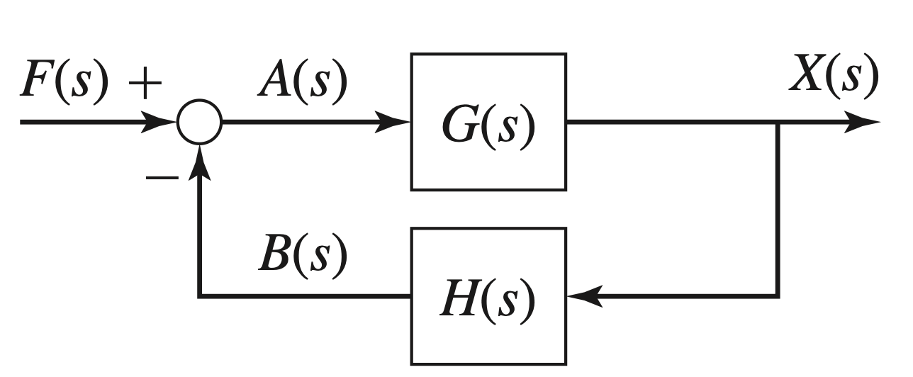
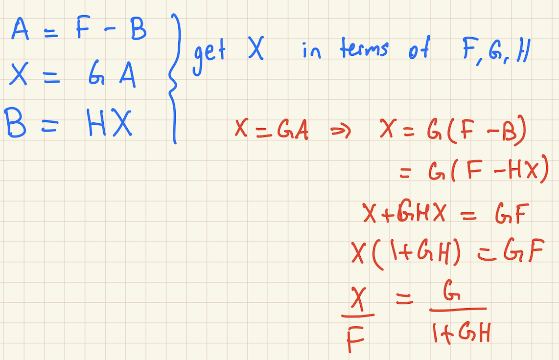
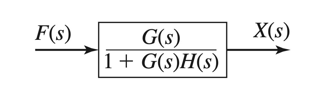
• Solution:

Examples of Equivalent Block Diagrams

The same underlying (linear physical) system can be represented as multiple block diagrams

Some are more helpful than others.

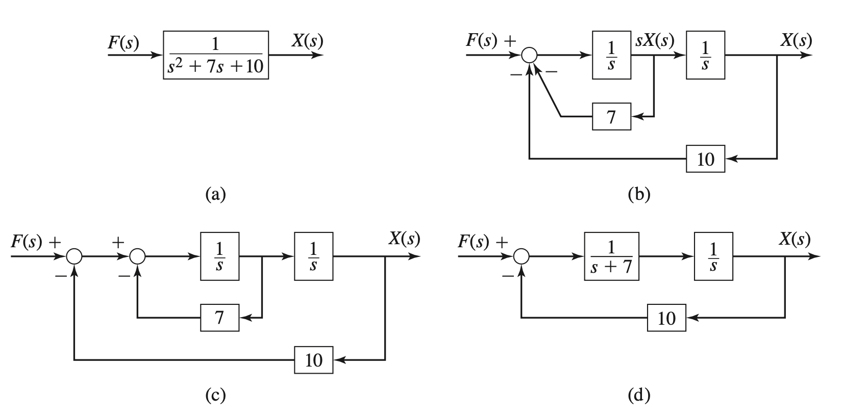
Finding Transfer Functions from block diagrams

• What is the transfer function for this system?
• There’s many different ones! \(\frac{X(s)}{F(s)}, \frac{X(s)}{G(s)}, \frac{Y(s)}{F(s)}, \frac{Y(s)}{G(s)}\)
• Procedure:
  1. Write down differential equations including intermediate variables
  2. Transform to Laplace space
  3. Eliminate the variables until the ones you want in the transfer function remain.

Worked Example: Find Transfer Function from block diagram

Coupled systems of equations

Recall that a system of two coupled (differential) equations is:

\[ \begin{aligned} \dot{x}_1 &= f_1(x_1,x_2,t) \\ \dot{x}_2 &= f_2(x_1,x_2,t) \end{aligned} \]

• How \(x_1\) changes depends on \(x_1\) and on \(x_2\)
• How \(x_2\) changes depends on \(x_2\) and on \(x_1\)
• If the equations are linear in \((x_1,x_2)\):

\[ \begin{aligned} \dot{x}_1 &= a x_1 + b x_2 + g_1(t) \\ \dot{x}_2 &= a x_1 + b x_2 + g_2(t) \end{aligned} \]

Block Diagram for a simple coupled system

Consider the coupled system of equations \[ \begin{aligned} \dot{x} + 7x &= y \\ \dot{y} + 5y &= g(t) \end{aligned} \tag{1}\]

• Block diagram for \(\dot{x} + 7x = f(t)\)
• In-class task: Represent Equation 1 with a block diagram.

• Solution

Why Block Diagrams are useful

\[ \begin{aligned} \dot{x} + 7x &= y \\ \dot{y} + 5y &= g(t) \end{aligned} \]

• Highlight the chain of causation from cause to effect
• Illustrate the interdependence between variables
• Allow for computer simulation systematically

Simplifying block diagrams

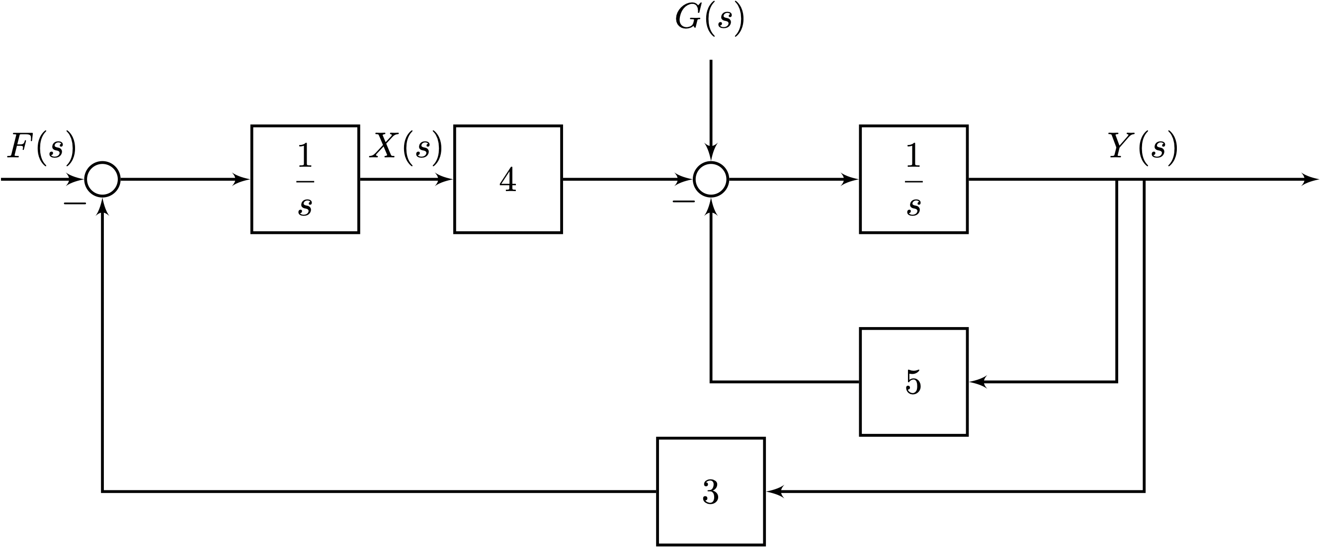
Block Diagrams with \(>1\) inputs

\[ \begin{aligned} \dot{x} &= -3y + f(t) \\ \dot{y} &= -5y + 4x + g(t) \end{aligned} \]

A coupled mechanical system