Lecture 15
E12 Linear Physical Systems Analysis
Equations of motion
Newton’s 2nd Law \[\sum F = m a\] gives rise to equations of motion.
We usually write equations of motion as second-order differential equations for the position
(or, sometimes, 1st-order differential equations for the velocity) of each constituent part of a mechanical system.
Free-Body Diagrams for Mechanical Systems
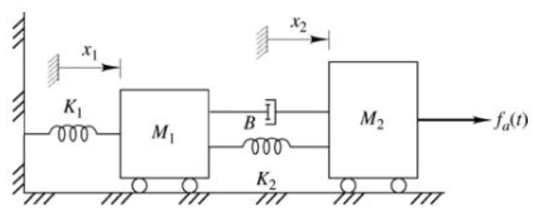
In-class activity Let’s determine the equations of motion for the following free-body diagram.
Questions to consider
- How many equations are needed?
- What is the order of the equations?
- How many state variables are there?
- Are the equations coupled?
- Are the equations linear?
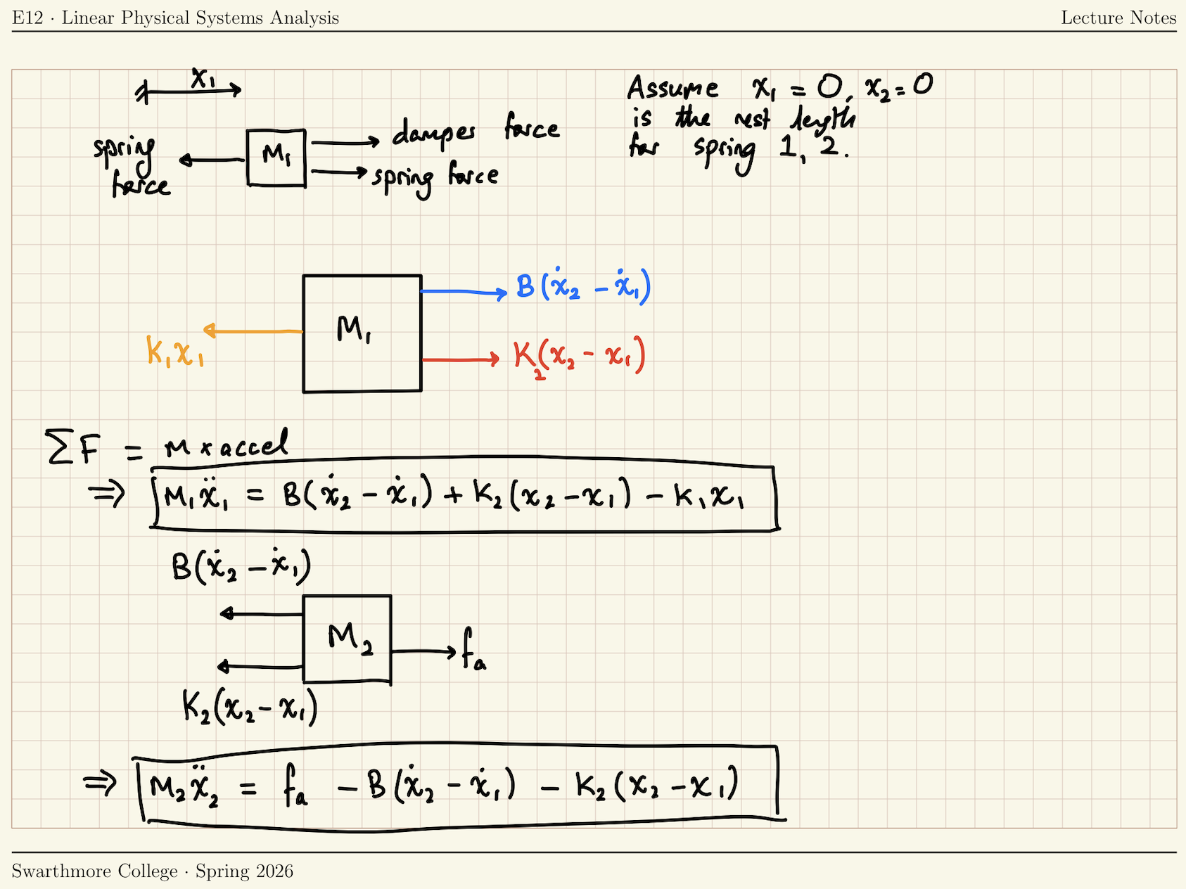
\[ M_1 \ddot{x}_1 + B \dot{x}_1 + (K_1+K_2) x_1 - B \dot{x}_2 - K_2 x_2 = 0 \tag{1}\]
\[ -B \dot{x}_1 - K_2 x_1 + M_2 \ddot{x}_2 + B \dot{x}_2 + K_2 x_2 = f_a(t) \tag{2}\]
Good checks (after bringing all terms to the same side):
- In the free-body diagram for mass 1, the sign of coefficients of \(x_1\) and its derivatives should be the same.
- In the free-body diagram for mass 2, the sign of coefficients of \(x_2\) and its derivatives should be the same.
Force input vs. Displacement inputs
The input to a mechanical system can either be provided as a prescribed force (function of time with units of Newtons), or as a prescribed displacement (function of time with units of meters).
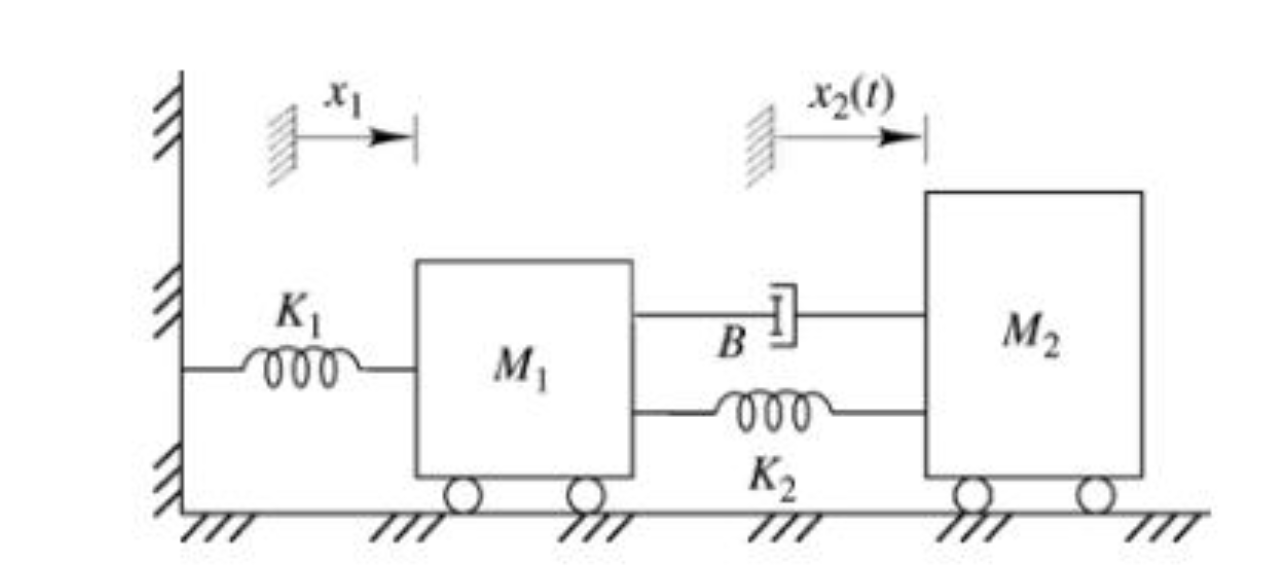
Because the displacement \(x_2(t)\) is prescribed in Figure 2,
- \(x_2(t)\) and its derivatives cease to be unknowns.
- We can make do with fewer equations
Writing the governing equations with displacement input
Alternative to Newton’s Law: d’Alembert’s Law
Newton’s 2nd Law can be written
\[\sum_i f_i = m \frac{dv}{dt}\]
d’Alembert’s Law is a restatement of Newton’s Law that makes use of a fictitious “inertial force” term.
\[\sum_i f_i - m \frac{dv}{dt} = 0\]
Where the term \(\displaystyle \boxed{- m \frac{dv}{dt}}\) is a fictitous force term.
With this definition of forces, d’Alembert’s Law states that, for an isolated system or body, \[ \sum_i f_i = 0 \]
where the forces \(f_i\) are understood to include fictitious forces.
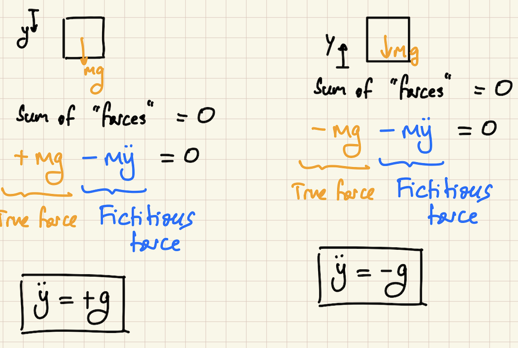
The Sign (Direction) of the fictitious inertial force term
When \(dv/dt > 0\), i.e., the object is accelerating in the positive \(x\) direction, the ‘inertial force’ acts in the negative \(x\) direction
Practice using d’Alembert’s Law
Use d’Alembert’s Law to determine the equation of motion for the following systems:


Force under prescribed displacements
We could ask the question: what force \(f(t)\) would have to be applied to mass 2 to give it precisely the displacement \(x_2(t)\) ?
Answer: use F.B.D. of Equation 2.
\[f_2 = -B \dot{x}_1 - K_2 x_1 + M_2 \ddot{x}_2 + B \dot{x}_2 + K_2 x_2 \tag{3}\]
\(f_2\) can easily be calculated by:
- Using Equation 1 to solve for \(x_1\) as a function of time
- We already know \(x_2\) and all its derivatives
- Plug in what we know about \(x_1\) and \(x_2\) into Equation 3.
If \(x_2(t)\) is specified to us as an input, then \(f_2(t)\), the force needed to bring about the displacement \(x_2(t)\) can be considered an output.
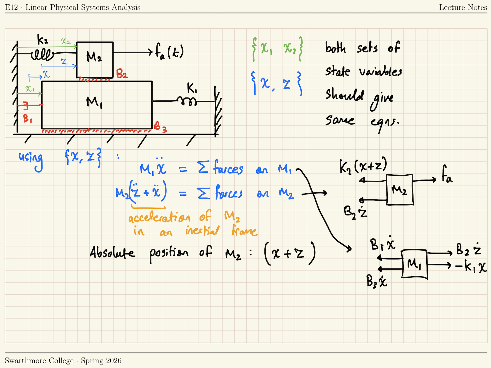
Measuring Displacement Relative to Another Displacement
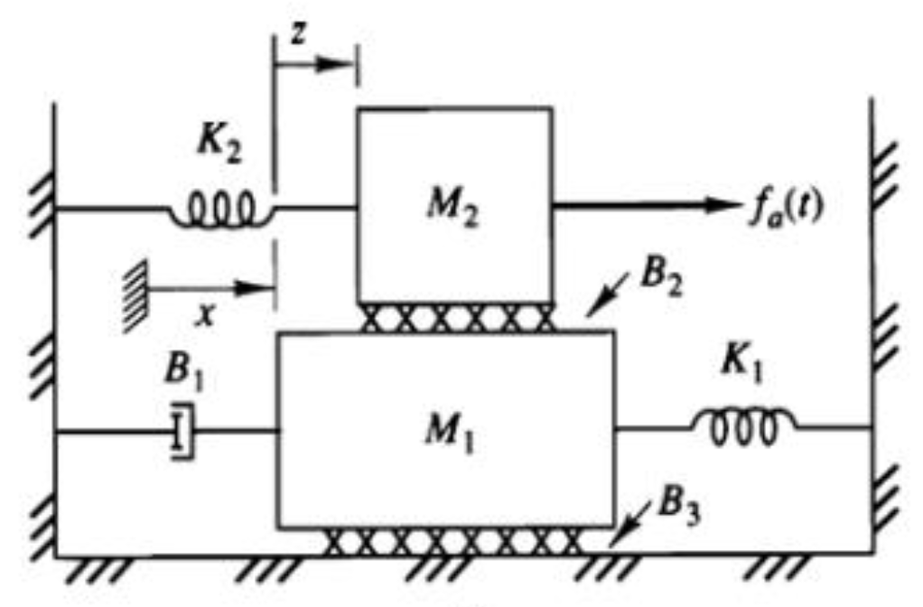
Find the equations of motion in terms of \(z\) and \(x\)
\[ \begin{aligned} M_2 \left( \ddot{z} + \ddot{x} \right) &= f_a(t) - B_2 \dot{z} - K_2 (z+x) \\ M_1 \ddot{x} &= -K_1 x -\left( B_1 + B_3 \right) \dot{x} + B_2 \dot{z} \end{aligned} \]
Equations of motion in terms of \(x_1\) and \(x_2\) measured from left wall:
\[ \begin{aligned} M_1 \ddot{x}_1 &= - K_1 x_1 - B_3 \dot{x}_1 - B_1 \dot{x}_1 - B_2 \left( \dot{x}_1 - \dot{x}_2 \right) \\ M_2 \ddot{x}_2 &= - K_2 x_2 - B_2 \left( \dot{x}_2 - \dot{x}_1 \right) + f_a(t) \end{aligned} \]