Problem Set 4 Solutions
ENGR 12, Spring 2026.
Solutions
1 The top-hat response
In this question we are interested in the response of an RC circuit to a ‘top-hat input’, i.e., an input function \(v_{\text{in}}(t)\) that looks like the top-hat function introduced in Lecture 7. We will proceed with a numerical approach.

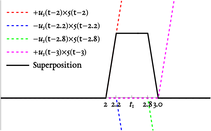
An RC circuit is powered by a voltage source that operates with the function \(f(t)\), where the function \(f(t)\) is given by the figure above, which is the superposition (a fancy word for ‘sum’) of the four shifted-and-rescaled ramp functions shown in the same figure.
The governing equations of this system are \[RC \dot{v} + v = v_{\text{in}}(t), \quad v(0) = 0.\]
The MATLAB script provided here allows you to generate the ‘hat response’ (i.e., the response of this system to an input shaped like the above figure) for different values of \(RC\).
% The hat function from class
function output = f1(t)
    % Builds a 'hat' centered at t = 2.5
    % using ramp functions.
    output = + heaviside(t-2).*5.*(t-2) + ...
             - heaviside(t-2.2).*5.*(t-2.2) + ...
             - heaviside(t-2.8).*5.*(t-2.8) + ...
             + heaviside(t-3).*5.*(t-3);
end

% Define a time domain with lots of values
N     = 1000;
tvals = linspace(0,8,N);

% Define RC values to use.
RCvals = [1,2,5];

% Define the right-hand side function of differential equation
function dvdt = rhs1(t,v,RC)
    dvdt = (f1(t) - v)/RC;
end

% Initial condition zero
x0 = 0;

% Call ode45 three times using three different values of RC.
[t1,x1] = ode45(@(t,x) rhs1(t,x,RCvals(1)), tvals, x0);
[t2,x2] = ode45(@(t,x) rhs1(t,x,RCvals(2)), tvals, x0);
[t3,x3] = ode45(@(t,x) rhs1(t,x,RCvals(3)), tvals, x0);

% Plot response
clf;
plot(tvals,f1(tvals),'--',"LineWidth",1,'Color',"green");  hold on;
plot(t1,x1,"LineWidth",2,"Color","blue");
plot(t2,x2,"LineWidth",2,"Color","red");
plot(t3,x3,"LineWidth",2,"Color","magenta");

legend("Input",sprintf("Output with RC = %.1f",RCvals(1)),...
               sprintf("Output with RC = %.1f",RCvals(2)),...
               sprintf("Output with RC = %.1f",RCvals(3)));

% Make it pretty
set(gca,"FontName","EB Garammond","FontSize",20);
xlabel("Time [seconds]");
ylabel("Voltage [ volts]");
grid on;

% Save to file
saveas(gcf,"hat-response.png");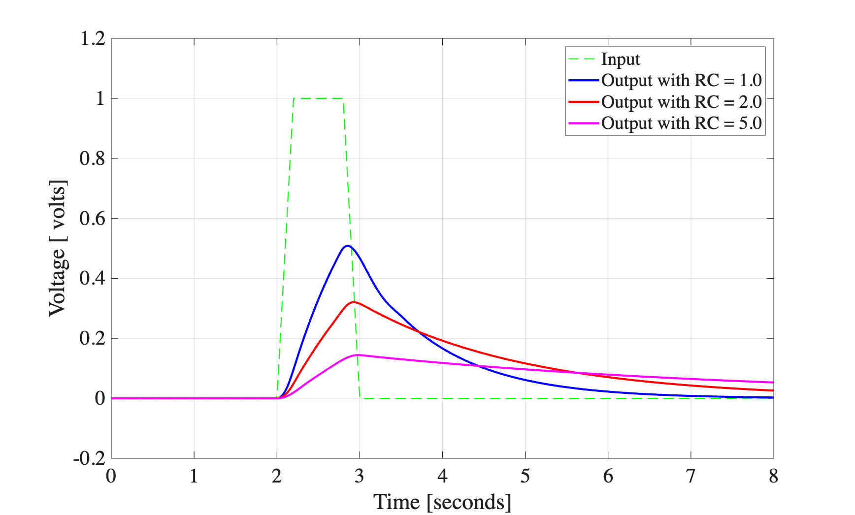
1.1 The ‘hat response and the time constant’
The values of \(RC\) currently shown in Figure 2 are not fully representative of all the different types of behaviors this system can show. Change the code to show three or four different values of \(RC\) (that may or may not include some of the currently-shown values; it’s up to you) that showcase the different types of behaviors you expect this system to have. Comment on your choices and describe what is happening using the RC circuit. In your comment and description/discussion, you should use the word ‘time constant’.
This question can be satisfactorily answered by generating a figure of the kind shown below.
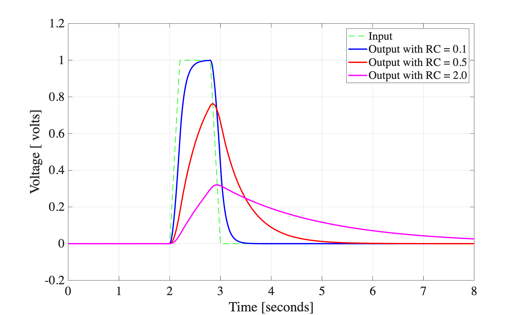
Because the duration of the ‘hat’ is about 1 second, it makes a great difference, qualitatively, whether the hat is applied to a system whose time constant is large compared to the duration of the hat, or small compared to the duration of the hat. We have thus chosen three values. At \(RC=0.1\), we find that the hat lasts much longer than the time constant of the system, and therefore the output has a chance of ‘catching up’ with the maximum value of the input, i.e., the capacitor has the chance to get fully charged by the voltage source before it shuts off. At \(RC=2.0\), on the other hand, the ‘hat’ only lasts for half of a time-constant, so the capacitor does not have enough time to charge before the input shuts off.
2 Time-shifted functions
2.1 Obtaining the expression for \(f(t)\)
Write down a mathematical expression, valid for all times \(t\), for the function of time shown below.
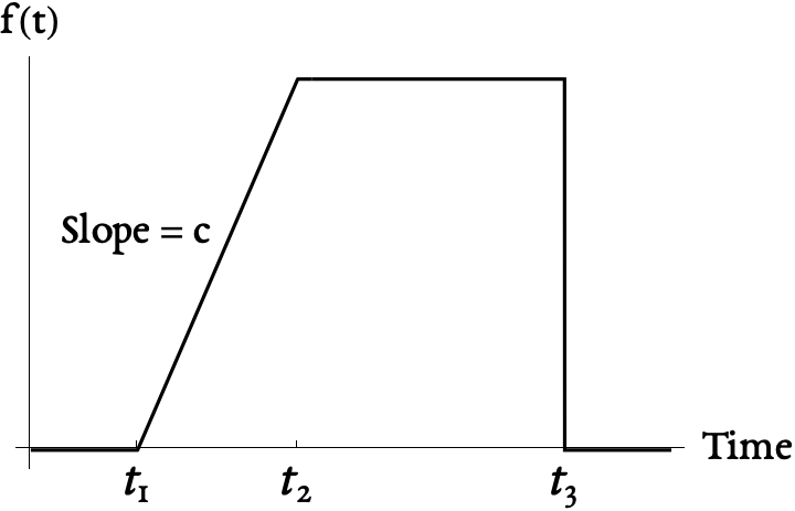
This function can be constructed using superposition of the following functions. 1. \[u_s(t - t_1) \cdot c \cdot (t-t_1)\] 2. \[-u_s(t - t_2) \cdot c \cdot (t-t_2)\] 3. \[-Au_s(t-t_3)\] where \(A\) must equal the height of the figure shown above, to ‘cancel it out’. If you squint at the figure long enough, you’ll see that \(A = c \cdot(t_2-t_1)\).
2.2 Laplace Transform
Determine an expression for \(F(s)\), the Laplace Transform of the function above. Write it down in two forms: as a rational function, and as a sum of fractions.
We have the following function of time: \[ f(t) = \underbrace{u_s(t - t_1) \cdot c \cdot (t-t_1)}_{f_1(t)} \underbrace{- u_s(t - t_2) \cdot c \cdot (t-t_2)}_{f_2(t)} \underbrace{- c \cdot(t_2-t_1) u_s(t-t_3)}_{f_3(t)} \] and we want to transform it to the \(s\) domain. To do this, we deal with three parts separately. Using the time-shifting property of Laplace Transforms, we can find
- Transform of \(f_1(t)\) \[ \begin{aligned} \mathcal{L}[f_1(t)] &= \mathcal{L}[u_s(t - t_1) \cdot c \cdot (t-t_1)] \\ &= e^{-st_1}\mathcal{L}[c \cdot t] \\ &= e^{-st_1} \frac{c}{s^2} \end{aligned} \]
- Transform of \(f_2(t)\) \[ \begin{aligned} \mathcal{L}[f_2(t)] &= \mathcal{L}[-u_s(t - t_2) \cdot c \cdot (t-t_2)] \\ &= e^{-st_2}\mathcal{L}[-c \cdot t] \\ &= e^{-st_2} \frac{-c}{s^2} \end{aligned} \]
- Transform of \(f_3(t)\) \[ \begin{aligned} \mathcal{L}[f_3(t)] &= \mathcal{L}[- c \cdot(t_2-t_1) u_s(t-t_3)] \\ &= e^{-st_3}\mathcal{L}[-c \cdot (t_2-t_1)] \\ &= e^{-st_3} \frac{-c \cdot (t_2-t_1)}{s} \end{aligned} \] Remember that the numerator of the fraction above is just a number, not a variable. Now, for the sum of fractions, we have \[ F(s) = e^{-st_1} \frac{c}{s^2} + e^{-st_2} \frac{-c}{s^2} + e^{-st_3} \frac{-c(t_2-t_1)}{s} \] And converting this to a rational function is pretty straightforward, since we know how to find the least common multiple of the denominators. We get \[ F(s) = \frac{e^{-st_1} c - e^{-st_2} c -s e^{-s t_3}(t_2-t_1) }{s^2} \]
2.3 Forced Response: Applying a time-shifted function to a circuit
An RC circuit is set up, as shown below, to which the input voltage is provided according to the following function of time: \[v_{\text{in}}(t) = u_s(t-t_1) \times k \times (t - t_1).\] Here, \(t_1\) is some positive constant and \(u_s\) is the Heaviside step function. Assume that \(RC\), the product of the resistance and capacitance, is some known number.
The capacitor is initially charged, and \(v(0) = v_0\), where \(v_0\) is some positive number.

Determine a mathematical expression for the free response and the forced response of the capacitor voltage in the frequency domain, and in the time domain.
Let’s write the governing equation in the time domain as \[ \begin{aligned} RC \dot{v} + v &= v_{\text{in}}(t) = u_s(t-t_1) k (t-t_1) \\ RC (s V - v(0)) + V &= \mathcal{L}[v_{\text{in}}(t)] = e^{-s t_1} \frac{k}{s^2} \\ RC s V + V& = e^{-s t_1} \frac{k}{s^2} + RC v(0) \\ V(s) &= \frac{1}{RCs+1} e^{-s t_1} \frac{k}{s^2} + \frac{RC v(0)}{RCs+1} \end{aligned} \] We now have our free and forced response in the frequency domain, i.e. \[ V(s) = \underbrace{\frac{1}{RCs+1} e^{-s t_1} \frac{k}{s^2}}_{\text{Forced Response}} + \underbrace{\frac{RC v_0}{RCs+1}}_{\text{Free Response}} \] Now, to put these two into the time domain, let’s start with the free response. In the frequency domain, we have \[ \frac{RC v_0}{RCs+1} = \frac{v_0}{s+1/RC} \] and from the table of Laplace transforms we know that in the time domain this is \[v_0 e^{-t/RC}.\] If we then look at the forced response, it’s a little more complicated. \[ \frac{1}{RCs+1} e^{-s t_1} \frac{k}{s^2} = e^{-s t_1} \frac{1/RC}{s + 1/RC} \frac{k}{s^2} \] and we can break this up into partial fractions with three terms: \[ e^{-s t_1} \frac{1/RC}{s + 1/RC} \frac{k}{s^2} = e^{-s t_1} \left( \frac{P}{s} + \frac{Q}{s^2} + \frac{R}{s+1/RC} \right) \] we then find the least common multiple of the denominators on the right hand side, and multiply the numerators accordingly to get \[ \begin{aligned} e^{-s t_1} \frac{1/RC}{s + 1/RC} \frac{k}{s^2} &= e^{-s t_1} \left( \frac{P}{s} + \frac{Q}{s^2} + \frac{R}{s+1/RC} \right) \\ &= e^{-s t_1} \left( \frac{Ps(s+1/RC) + Q(s+1/RC) + Rs^2}{s^2 (s+1/RC)}\right) \end{aligned} \] now, the numerator on the right hand side has terms with \(s\), terms with \(s^2\), and terms without any \(s\). We can equate the numerator of the right hand side with the numerator on the left hand side, term by term, to write \[ \begin{aligned} 0s^2 &= (P + R)s^2 \\ 0s &= Ps/RC + Qs \\ k/RC &= Q/RC \end{aligned} \] Thus, we find that \(Q = k\), \(P=-k RC\), and \(R = + k RC\). We can now put together the forced response as a sum of fractions \[ e^{-s t_1} \left( \frac{-k RC}{s} + \frac{k}{s^2} + \frac{k RC}{s+1/RC} \right) \] The next task is to put these into the time domain by looking closely at the table of Laplace Transforms. From the table, we know that \[ \begin{aligned} &\mathcal{L}^{-1} \left[ \frac{-kRC}{s}\right] = -k RC \\ &\mathcal{L}^{-1} \left[ \frac{k}{s^2}\right] = k t \\ &\mathcal{L}^{-1} \left[ \frac{kRC}{s+1/RC}\right] = k RC e^{-t/RC} \end{aligned} \] and by the time-shifting property, \[ \begin{aligned} &\mathcal{L}^{-1} \left[ e^{-s t_1 } \frac{-kRC}{s}\right] = -k RC u_s(t-t_1) \\ &\mathcal{L}^{-1} \left[ e^{-s t_1 } \frac{k}{s^2}\right] = k (t-t_1) u_s(t-t_1) \\ &\mathcal{L}^{-1} \left[ e^{-s t_1 } \frac{kRC}{s+1/RC}\right] = k RC e^{-(t-t_1)/RC}u_s(t-t_1) \end{aligned} \] which is a fancy way of saying that ‘The inverse-Laplace transform of a \(e^{-sD}\) times a function equals the inverse-Laplace transform of that function shifted forward by \(D\) units of time’.
So the forced response in the time domain is the sum of the above three terms. \[ -k RC u_s(t-t_1) + k (t-t_1) u_s(t-t_1) + k RC e^{-(t-t_1)/RC}u_s(t-t_1) \]
3 Basic Block Diagrams
3.1 One input, one output
Consider the system represented by the following diagram.
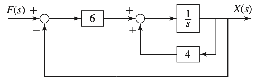
- Determine the transfer function \(X(s)/F(s)\).
- Draw a simplified version of this block diagram in which there are only two block elements.
- Draw a simplified version of this block diagram in which there is only one block element.
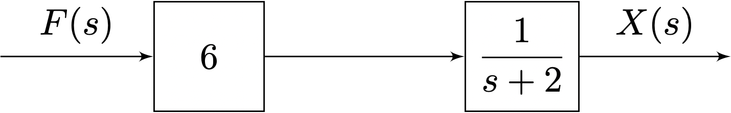
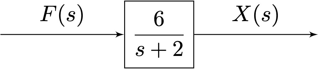
The above block diagram says: \[sX = 4X + 6(F-X)\] This can of course be simplified to get \[ \begin{aligned}sX &= 4X + 6(F-X) \\ \implies s X &= 4X + 6F - 6X \\ sX + 2X &= 6F \\ X(s+2) &= 6F \\ \frac{X}{F} &= \boxed{\frac{6}{s+2}} \end{aligned} \] Thus, the transfer function between the input \(F\) and the output \(X\) is \(1/(s+2)\). The following two block diagrams also work for this purpose.
3.2 Two inputs, one output
Consider the system represented by the following diagram.
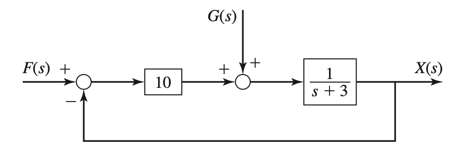
- Determine the transfer function \(X(s)/F(s)\)
- Determine the transfer function \(X(s)/G(s)\)
We can interpret this diagram with the equation \[ \begin{aligned} X &= \frac{1}{s+3} \left( G+10 (F-X)\right) \\ &= \frac{1}{s+3} \left( G + 10F - 10X \right) \\ sX + 3X + 10X &= G + 10F \\ (s+ 13)X &= G + 10F \\ X = \frac{1}{s+13}G + \frac{10}{s+13} F \end{aligned} \] Thus, the two transfer functions we are looking for are:
- From \(G\) to \(X\): \(\displaystyle \frac{1}{s+13}\)
- From \(F\) to \(X\): \(\displaystyle \frac{10}{s+13}\)
3.3 Block Diagram from equations
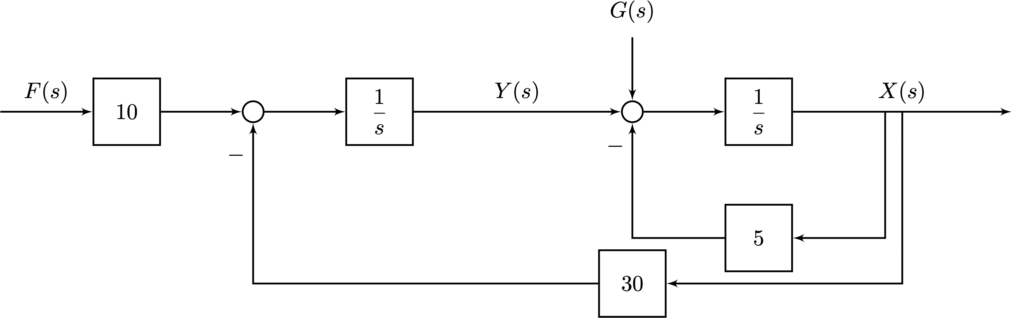
Draw a block diagram for the following system. The output is \(x(t)\) or \(X(s)\), and the inputs are \(f(t)\) and \(g(t)\) in the time domain, i.e., \(F(s)\) and \(G(s)\) in the frequency domain. Also indicate on your diagram the location of \(Y(s)\).
\[ \begin{aligned} \dot{x} &= y - 5x + g(t) \\ \dot{y} &= 10 f(t) - 30x \end{aligned} \]
The block diagram looks like this
4 Coupled systems and block diagrams
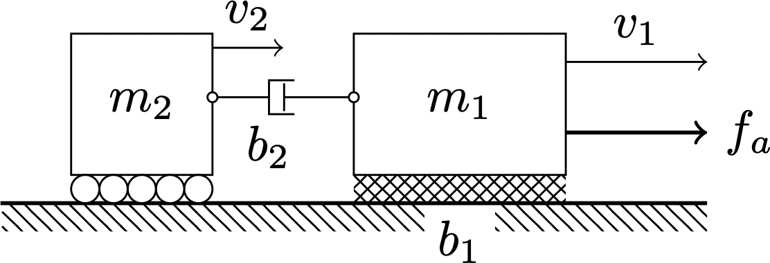
4.1 A Mechanical System
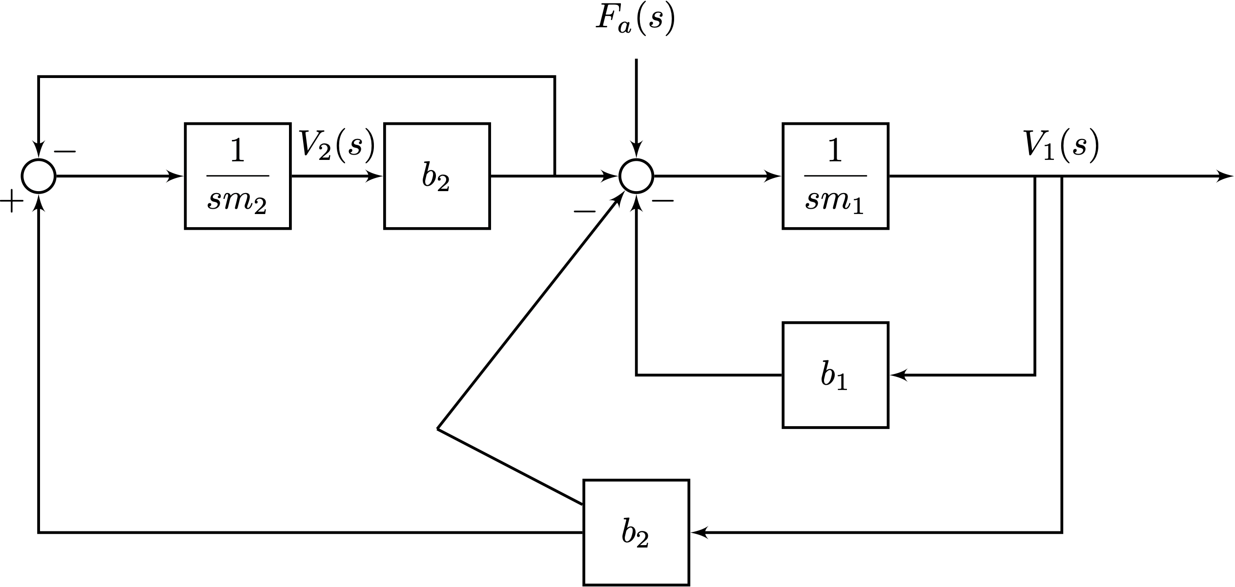
In class, it was shown that the governing equations for the following system of masses and friction elements is
\[ \begin{aligned} m_1 \dot{v}_1 + b_1 v_1 &= f_1 - b_2 v_1 + b_2 v_2 \\ m_2 \dot{v}_2 \phantom{+ b_1 v_1} &= \phantom{f_1 -} b_2 v_1 - b_2 v_2 \end{aligned} \]
The system is shown below.
Use the following block diagram to represent the system above. The ‘?’ symbols indicate inputs and outputs.
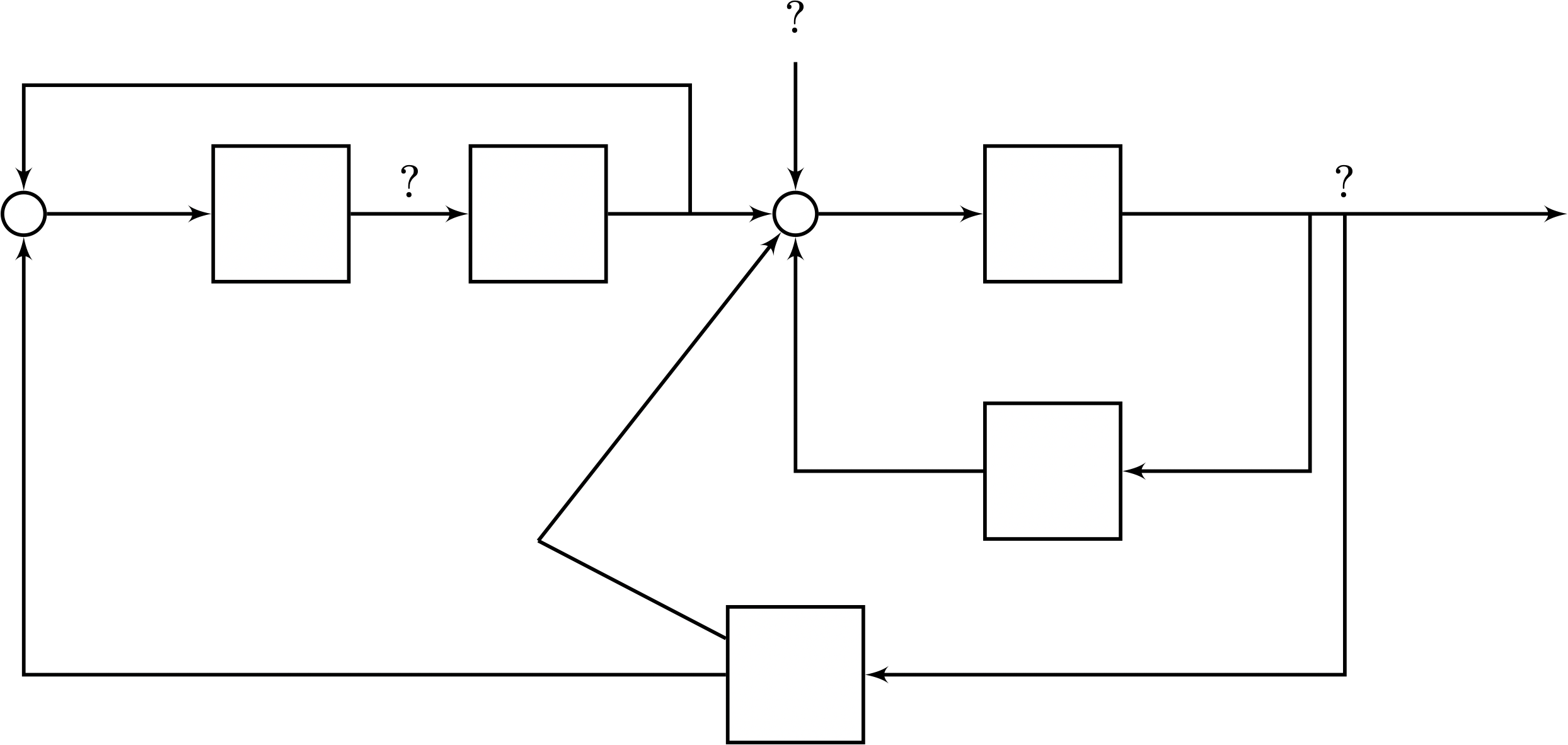
The system can be represented by the following block diagram.
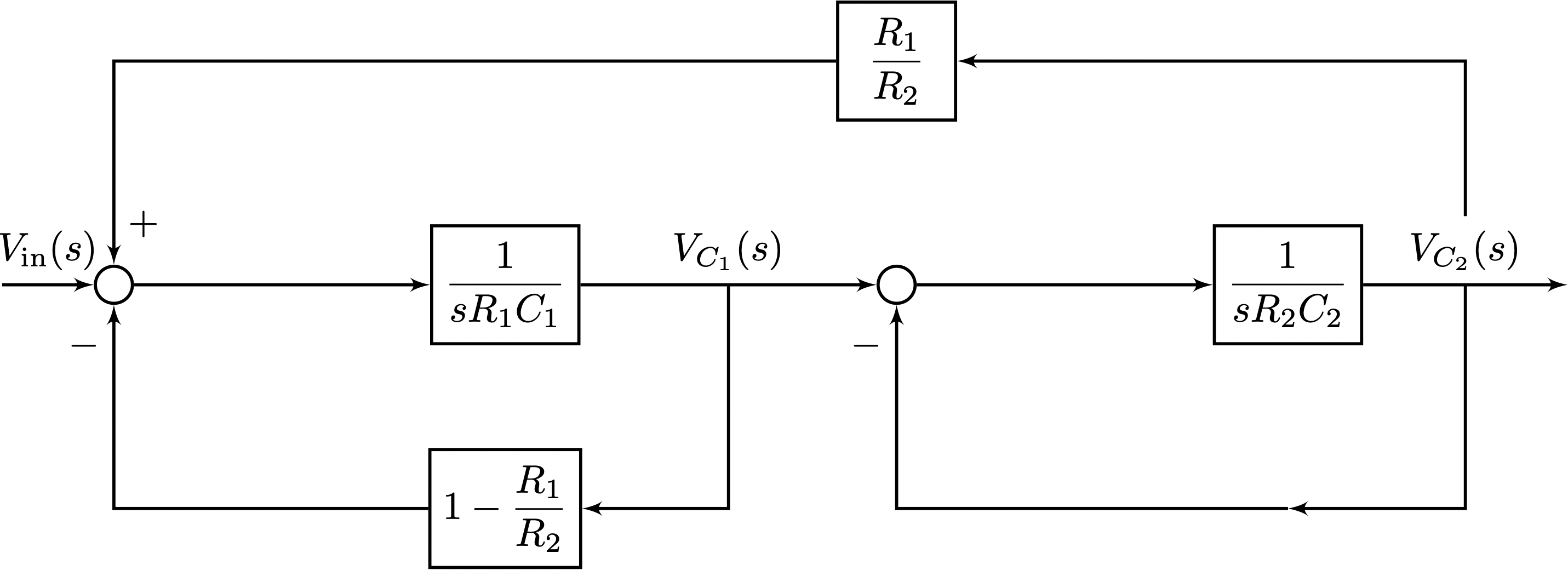
4.2 An Electrical System
Consider the circuit shown below.

- Write down a set of coupled differential equations for the voltage across capacitor \(C_1\), \(v_{C_1}\) and the voltage across the capacitor \(C_2\), \(v_{C_2}\).
The governing equations for this circuit can be found by applying Kirchhoff’s Laws as below.
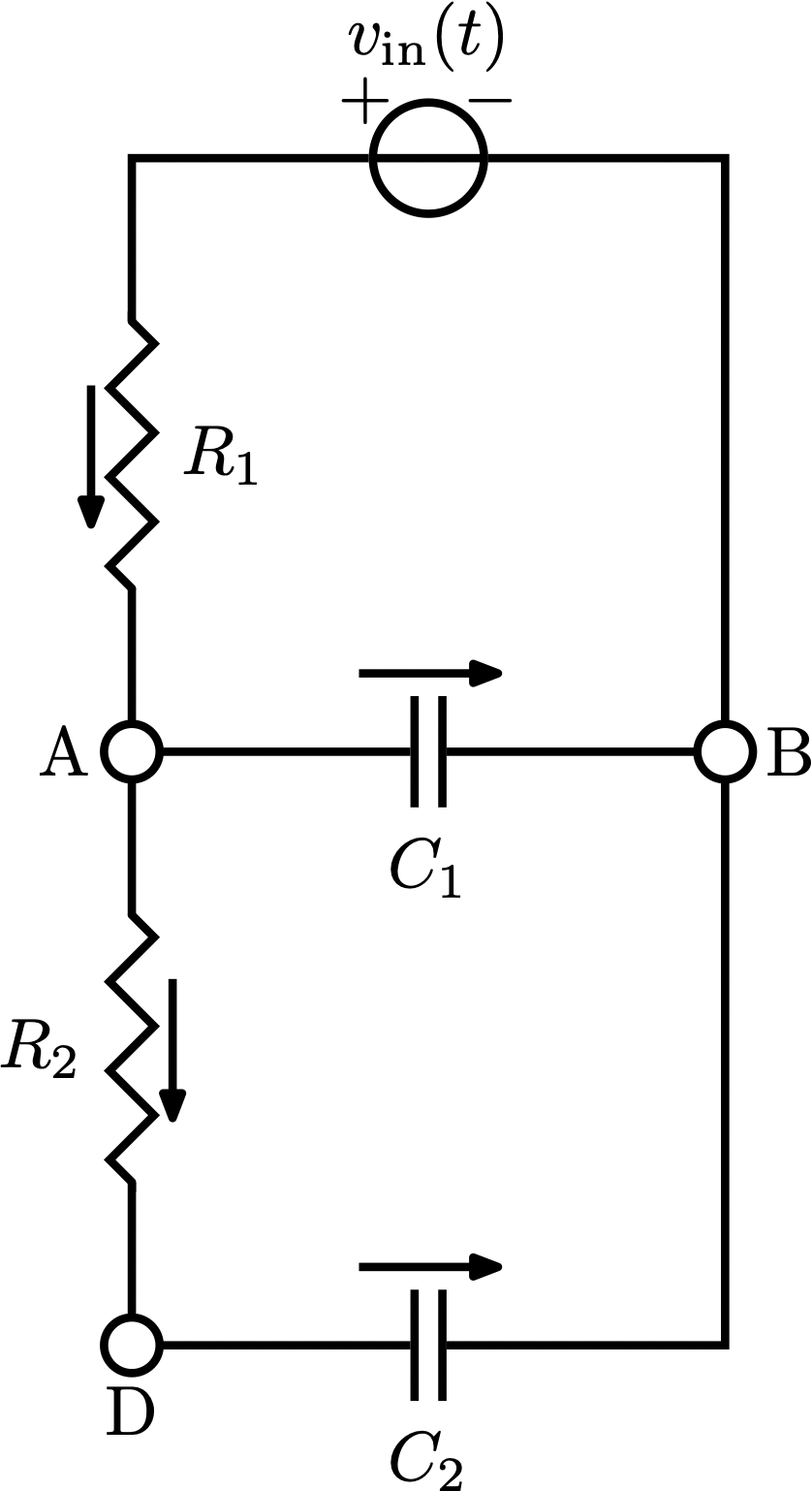
Apply Kirchhoff’s Voltage Law to write three equations, which we may or may not use. \[ \begin{aligned} v_{\text{in}} - v_{R_1} - v_{C_1} &= 0 \\ v_{\text{in}} - v_{R_1} - v_{R_2} - v_{C_2} &= 0 v_{\text{in}} - v_{R_2} - v_{C_2} &= 0 \end{aligned} \]
Apply Kirchhoff’s Current Law at node D to learn that \[ \begin{aligned} i_{R_2} &= i_{C_2} \\ \frac{v_{R_2}}{R_2} &= C_2 \frac{dv_{C_2}}{dt} \\ \frac{v_{C_1} - v_{C_2}}{R_2} &= C_2 \frac{dv_{C_2}}{dt} \\ R_2 C_2 \dot{v}_{C_2} &= v_{C_1} - v_{C_2} \\ R_2 C_2 \dot{v}_{C_2} + v_{C_2} &= v_{C_1} \end{aligned} \]
Apply Kirchhoff’s Current Law at node A to learn that \[ \begin{aligned} i_{R_1} &= i_{R_2} + i_{C_1} \\ \frac{v_{R_1}}{R_1} &= \frac{v_{R_2}}{R_2} + C_1 \frac{dv_{C_1}}{dt} \\ \frac{v_{\text{in}} - v_{C_1}}{R_1} &= \frac{v_{C_1} - v_{C_2}}{R_2} + C_1 \frac{dv_{C_1}}{dt} \\ \implies \frac{v_{\text{in}} - v_{C_1}}{R_1} - \frac{v_{C_1} - v_{C_2}}{R_2} &= C_1 \dot{v}_{C_1} \\ \frac{R_2 (v_{\text{in}} - v_{C_1}) - R_1(v_{C_1} - v_{C_2})}{R_1 R_2} &= C_1 \dot{v}_{C_1} \\ R_1 C_1 \dot{v}_{C_1} &= v_{\text{in}} - v_{C_1} - \frac{R_2}{R_1} (v_{C_1}-v_{C_2}) \\ R_1 C_1 \dot{v}_{C_1} &= v_{\text{in}} - \left( 1 - \frac{R_1}{R_2} \right) v_{C_1} + \frac{R_1}{R_2} v_{C_2} \\ R_1 C_1 \dot{v}_{C_1} + \left( 1 - \frac{R_1}{R_2} \right) v_{C_1} &= v_{\text{in}} + \frac{R_1}{R_2} v_{C_2} \end{aligned} \]
We now have our two equations, both in the suggested form. They are
\[ \boxed{ \begin{aligned} R_2 C_2 \dot{v}_{C_2} + v_{C_2} &= v_{C_1} \\ R_1 C_1 \dot{v}_{C_1} + \left( 1 - \frac{R_1}{R_2} \right) v_{C_1} &= v_{\text{in}} + \frac{R_1}{R_2} v_{C_2} \end{aligned} } \]
- Draw a block diagram illustrating this system.