Problem Set 7 Solutions

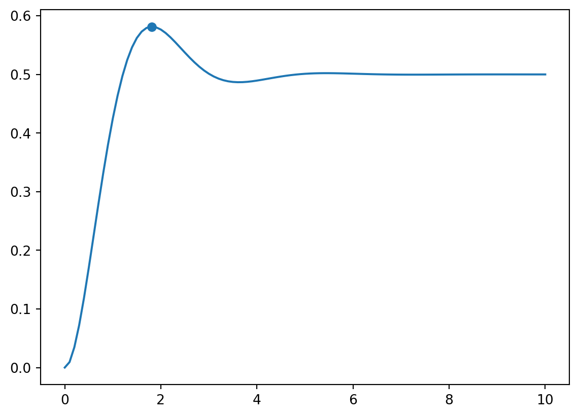
ENGR 12, Spring 2026.

Solutions

1 Classifying second-order systems

1.1 Under-, over- and critically- damped systems

For each of the following systems, determine if you expect the free response to be over-damped, under-damped, or critically damped. Show your work. If a system does not seem to fall into any category, sketch the shape you expect its solution \(x(t)\) to take.

1. \[\ddot{x} + 4 \dot{x} + 3 x = 0\]

TipSolution

\[\frac{-b \pm \sqrt{b^2-4mk}}{2m} = \frac{-4 \pm \sqrt{4^2-4\cdot 1 \cdot 3}}{2} = \frac{-4 \pm \sqrt{4}}{2} = \{ -1,-3\}\]

Therefore, the roots of the characteristic polynomial are real, distinct, and negative, and we expect the system’s free response to be overdamped.

2. \[\ddot{x} + 3 \dot{x} + 4 x = 0\]

TipSolution

\[\frac{-b \pm \sqrt{b^2-4mk}}{2m} = \frac{-3 \pm \sqrt{3^2-4\cdot 1 \cdot 4}}{2} = \frac{-4 \pm \sqrt{9-16} }{2} = -2 \pm \frac{\sqrt{7}}{2} i\]

Therefore, the roots of the characteristic polynomial are complex and distinct, with real part negative. Thus, we expect the system’s free response to be underdamped.

3. \[2\ddot{x} + \dot{x} + 3 x = 0\]

TipSolution

\[\frac{-b \pm \sqrt{b^2-4mk}}{2m} = \frac{-1 \pm \sqrt{1^2-4\cdot 2 \cdot 3}}{2 \cdot 2} = \frac{1}{4} \left( -1 \pm \sqrt{-23}\right) = \frac{1}{4} \left( -1 \pm i \sqrt{23}\right) \]

Therefore, the roots of the characteristic polynomial are complex and distinct, with real part negative. Thus, we expect the system’s free response to be underdamped.

4. \[3\ddot{x} + 6\dot{x} + 3 x = 0\]

TipSolution

\[\frac{-b \pm \sqrt{b^2-4mk}}{2m} = \frac{-6 \pm \sqrt{6^2-4\cdot 3 \cdot 3}}{2 \cdot 3} = \frac{-6 \pm \sqrt{0}}{6} = \{ -1, -1 \}\]

Therefore, the roots of the characteristic polynomial are negative, real and repeated. Thus, we expect the system’s free response to be critically damped.

5. \[ \ddot{x} + 4\dot{x} -3 x = 0\]

TipSolution

\[ \begin{aligned} \frac{-b \pm \sqrt{b^2-4mk}}{2m} = \frac{-4 \pm \sqrt{4^2-4\cdot 1 \cdot (-3)}}{2} &= \frac{-4 \pm \sqrt{28}}{2} \\ &= -2 \pm \sqrt{7} \end{aligned} \]

Therefore, one of the roots of the characteristic polynomial is negative, and the other root is positive. This does not fall into one of the categories of underdamped, overdamped, or critically damped.

We expect this to look approximately like one of the following solutions, depending on the initial conditions.

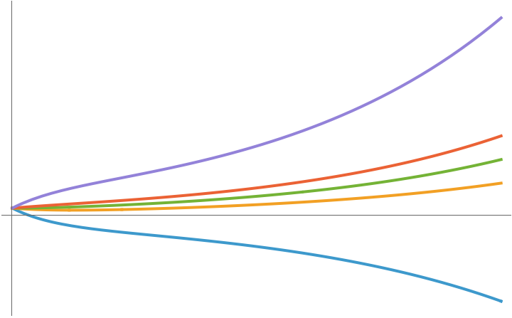
The key feature to note here is that \(x\) goes off to infinity (positive or negative).

6. \[2\ddot{x} - 4\dot{x} +3 x = 0\]

TipSolution

\[ \begin{aligned} \frac{-b \pm \sqrt{b^2-4mk}}{2m} = \frac{-(-4) \pm \sqrt{(-4)^2-4 \cdot 2 \cdot 3}}{2 \cdot 2} &= \frac{4 \pm \sqrt{16-24}}{4} \\ &= \frac{1}{4} \left( 4 \pm i \sqrt{8} \right) \end{aligned} \]

Therefore, the roots of the characteristic polynomial are complex, and their real part is positive. This too does not fall into one of the categories of underdamped, overdamped, or critically damped.

We expect this to look approximately like the following solutions.

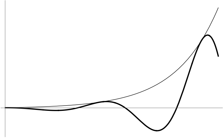
Here, too \(x\) goes off to infinity.

2 Forced (Step) Response of second-order systems

Spring-mass-damper system. Assume that \(x\) has been chosen such that when \(x=0\), there is no push or pull in the spring.

2.1 Deriving an expression for the step response

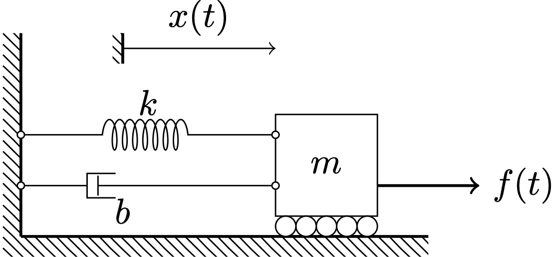
Show that the forced response of a spring-mass-damper system, such as the one shown above, to a ‘step function force’ equal to \(c\), i.e., the solution of the differential equation \[m \ddot{x} + b \dot{x} + k x = c u_s(t), \tag{1}\] is \[x(t) = \frac{c}{ m \left( r^2+\omega^2 \right)} \left[ 1 - e^{rt} \left( \cos \omega t - \frac{r}{\omega} \sin \omega t \right) \right]. \tag{2}\] Here, \(r\) is the real part of the roots of the characteristic polynomial, and \(\omega\) the imaginary part of the roots of the characteristic polynomial. You do not need to expand \(r\) and \(\omega\) in terms of \(m\), \(b\) and \(k\) in your answer.

In the process of showing the above, also write down the frequency-domain expression for the forced response, i.e., write down an expression for \(X(s)\) in terms of \(\omega\), \(r\) and \(c\).

TipSolution

Let’s start by taking the Laplace Transform of Equation 1.

\[ \begin{aligned} \mathcal{L} \left[ m \ddot{x} + b \dot{x} + k x \right] &= \mathcal{L} \left[ c u_s(t)\right] \\ m s^2 X + b s X + k X &= \frac{c}{s} \end{aligned} \] Then we rearrange the equation to solve for \(X(s)\) and find: \[ X(s) = \frac{c}{s} \frac{1}{m s^2 + b s + k} \]

Next, we note that when the roots of \(m s^2 + bs + k\) are complex — as they must be in the underdamped case — they can be written as \(s_{1,2} = r \pm i \omega\) and then we have \[ \begin{aligned} m s^2 + bs + k = m(s-s_1)(s-s_2) &= m(s - r - i \omega) (s - r + i \omega) \\ &= m \left[ (s-r)^2 + \omega^2 \right] \end{aligned} \] where \(r,\omega\) are the real and imaginary parts of the roots of the characteristic polynomial. Let’swrite down what these two terms actually are: \[r = -\frac{b}{2m}, \quad \omega = \frac{1}{2m}\sqrt{4mk-b^2}.\] For convenience, we can take the \(m\) to the other side like so: \[ \begin{aligned} X(s) = \frac{c}{s} \frac{1}{m s^2 + b s + k} &= \frac{c}{s} \frac{1}{m \left[ (s-r)^2 + \omega^2 \right]} \\ \implies m X(s) &= \frac{c}{s} \frac{1}{(s-r)^2 + \omega^2}. \end{aligned} \]

We would now like to write this as the sum of some fractions that look like the entries in the Laplace Transform table. As suggested by the hint given to us, we will use the following partial-fraction decomposition: \[ m X(s) = \frac{c}{s} \frac{1}{(s-r)^2 + \omega^2} = \frac{P}{s} + Q \frac{s-r}{(s-r)^2+\omega^2} + R \frac{\omega}{(s-r)^2+\omega^2} \tag{3}\]

Then, using the least common multiple of the denominators of the partial fractions in Equation 3, we can write that \[ \begin{aligned} m X(s) = \frac{c}{s} \frac{1}{(s-r)^2 + \omega^2} &= \frac{P}{s} + Q \frac{s-r}{(s-r)^2+\omega^2} + R \frac{\omega}{(s-r)^2+\omega^2} \\ &= \frac{P \left( (s-r)^2+\omega^2 \right) + Q (s-r)s + R \omega s }{s \left( (s-r)^2+\omega^2 \right)} \end{aligned} \]

We are now in a position to compare the numerators of the two sides of the following equation

\[ \begin{aligned} \frac{c}{s} \frac{1}{(s-r)^2 + \omega^2} &= \frac{P \left( (s-r)^2+\omega^2 \right) + Q (s-r)s + R \omega s }{s \left( (s-r)^2+\omega^2 \right)} \\ \implies c &= P (s^2 - 2 r s + r^2 + \omega^2 ) + Q s^2 - r s Q + R \omega s \end{aligned} \]

• Equating \(s^2\) terms, we find that \(P + Q = 0\)
• Equating \(s^1\) terms, we find that \(-2 P r - Q r + R \omega = 0\)
• Equating \(s^0\) terms, we find that \(P r^2 + P \omega^2 = c\)

Thus, we can solve the above equations simultaneously to learn that \[P = \frac{c}{r^2 + \omega^2}\] \[Q = \frac{-c}{r^2 + \omega^2}\] \[R = \frac{r}{\omega} \frac{c}{r^2 + \omega^2}\]

Thus, \(mX(s)\) can be written as the sum of three terms:

\[m X(s) = \overbrace{\left( \frac{c}{r^2+\omega^2} \right)}^{P} \frac{1}{s} + \overbrace{\left( \frac{-c}{r^2 + \omega^2} \right)}^{Q} \frac{s-r}{(s-r)^2+\omega^2} + \overbrace{\left( \frac{r}{\omega} \frac{c}{r^2 + \omega^2} \right)}^{R} \frac{\omega}{(s-r)^2+\omega^2} \tag{4}\]

Now, we look at the relevant entries in the table of Laplace Transform pairs. Specifically, entries 10 and 11 state that

\[\mathcal{L}^{-1} \left[ \frac{b}{(s+a)^2 + b^2} \right] = e^{-at} \sin b t\] \[\mathcal{L}^{-1} \left[ \frac{s+a}{(s+a)^2 + b^2} \right] = e^{-at} \cos b t\]

Thus, the term multiplying \(Q\) in Equation 4 can be transformed to the time domain using

\[\mathcal{L}^{-1} \left[ \frac{s-r}{(s-r)^2 + \omega^2} \right] = e^{rt} \cos \omega t\]

and the term multiplying \(R\) in Equation 4 can be transformed to the time domain using

\[\mathcal{L}^{-1} \left[ \frac{\omega}{(s-r)^2 + \omega^2} \right] = e^{rt} \sin \omega t.\]

The term multiplying \(P\) can be transformed using \[\mathcal{L}^{-1} \left[ \frac{1}{s}\right] = u_s(t),\] into the unit step function.

Thus, in the time domain, Equation 4 can be written as

\[m x(t) = \left( \frac{c}{r^2+\omega^2} \right) u_s(t) + \left( \frac{-c}{r^2 + \omega^2} \right) e^{rt} \cos \omega t + \left( \frac{r}{\omega} \frac{c}{r^2 + \omega^2} \right) e^{rt} \sin \omega t\]

Taking \(c(r^2+\omega^2)^{-1}\) as a common factor and restricting \(x(t)\) to \(t>0\) (which allows us to replace \(u_s(t)\) with the number ‘\(1\)’, we get

\[m x(t) = \frac{c}{r^2 + \omega^2} \left( 1 - e^{rt} \cos \omega t + \frac{r}{\omega} e^{rt} \sin \omega t \right)\]

which can be simplified to give

\[x(t) = \frac{c}{m \left( r^2+\omega^2 \right)} \left[ 1 - e^{rt} \left( \cos \omega t - \frac{r}{\omega} \sin \omega t \right) \right],\] identical to Equation 2, Q.E.D.

2.2 Using specific numbers.

For this part, it is OK to just use Equation 2 directly without having to solve any equations.

2.2.1 Expression for \(x(t)\) with numbers

For \(m =1, b = 2, k = 4\) and \(c=2\), write down the expression for \(x(t)\) using numbers and functions. There should be no free parameters here.

TipSolution

The roots of the characteristic polynomial \(m s^2 + b s + k\) are given by the quadratic formula, \[s_{1,2} = \frac{-b \pm \sqrt{b^2 - 4mk}}{2m}.\] Plugging in the values above, we get \(s_{1,2} = -1 \pm i \sqrt{3}\). Therefore, \(r=-1\) and \(\omega = \sqrt{3}\).

\[ x(t) = \frac{2}{(-1)^2+\sqrt{3}^2} \left[ 1 - e^{-t} \left( \cos \sqrt{3} t - \frac{-1}{\sqrt{3}} \sin \sqrt{3} t \right) \right] \] \[ = \frac{1}{2} \left[ 1 - e^{-t} \left( \cos \sqrt{3} t + \frac{1}{\sqrt{3}} \sin \sqrt{3} t \right) \right] \tag{5}\]

2.2.2 Predicting the steady-state response

Recall that the ‘steady-state response’ to an input is how a system behaves in the long run due to the input it receives. For \(m =1, b = 2, k = 4\) and \(c=2\), calculate — without making a plot — the steady-state response, i.e. what value(s) \(x(t)\) takes in the long run.

TipSolution

Notice that when \(t \rightarrow \infty\), \(e^{-rt} \rightarrow 0\). So the term inside the parantheses in Equation 5 goes to zero at long times. The only remaining term is, therefore, \(\frac{1}{2}\). The steady-state value of \(x(t)\) is expected to be \(\frac{1}{2}\).

2.2.3 Making a plot

1. For \(m =1, b = 2, k = 4\) and \(c=2\), make a plot of \(x(t)\) for the first ten seconds.
2. Either using your plot or using math, determine the time at which the spring is the farthest from its original position, and write the value of \(t\) and of \(x\) for this instant.

TipSolution

1. The plot can be produced using any plotting software.

from numpy import sqrt,sin,cos,exp,linspace,pi
from matplotlib.pyplot import plot,scatter

t = linspace(0,10,101)
x = 0.5*(1 - exp(-t)*(cos(sqrt(3)*t) + (1/sqrt(3))*sin(sqrt(3)*t)))
plot(t,x)
scatter(pi/sqrt(3),0.5815)

Let’s use math. We would like to look for turning points in the graph of \(x(t)\), so let’s take the derivative.

\[ \begin{aligned} x &= \frac{c}{r^2+\omega^2} \left[ 1 - e^{rt} \left( \cos \omega t - \frac{r}{\omega} \sin \omega t \right) \right] \\ \frac{dx}{dt} &= - \frac{c}{r^2+\omega^2} \left [ e^{rt} \left( -\omega \sin \omega t - r \cos \omega t \right) + r e^{rt} \left( \cos \omega t - \frac{r}{\omega} \sin \omega t\right)\right] \\ &= - \frac{c}{r^2+\omega^2} \left [ e^{rt} \left( -\omega \sin \omega t - \cancel{r \cos \omega t} \right) + e^{rt} \left( \cancel{r \cos \omega t} - \frac{r^2}{\omega} \sin \omega t\right)\right] \\ &= - \frac{c}{r^2 + \omega^2} e^{rt} \left[ - \omega \sin \omega t - \frac{r^2}{\omega} \sin \omega t\right] \\ &= \frac{c}{r^2 + \omega^2} e^{rt} \sin \omega t \left[ \omega + \frac{r^2}{\omega}\right] \\ &= \frac{c}{\cancel{r^2 + \omega^2}} e^{rt} \sin \omega t \left[ \frac{\cancel{\omega^2 + r^2}}{\omega}\right] \\ &= \frac{c}{\omega} e^{rt} \sin \omega t \end{aligned} \]

To find extrema, we have to equate this to zero, so we get the equation \[\frac{c}{\omega} e^{rt} \sin \omega t = 0\] The above equation is true whenever \(\omega t = 0, \pi, 2\pi, 3\pi,...\) but we are interested in the case when \(\omega t = \pi\). Thus, \(\boxed{t = \pi/\omega \approx 1.814}\) is the time we are looking for. Plugging this into the expression for \(x\), we find that the farthest distance traveled by the mass is \[ \begin{aligned} x &= \frac{c}{r^2+\omega^2} \left[ 1 - e^{r{\pi}/{\omega}} \left( \cos \pi - \frac{r}{\omega} \sin \pi \right) \right] \\ &= \frac{c}{r^2+\omega^2} \left[ 1 - e^{r{\pi}/{\omega}} \left( \cancelto{-1}{\cos \pi} - \frac{r}{\omega} \cancelto{0}{\sin \pi} \right) \right] \\ &= \frac{c}{r^2+\omega^2} \left[ 1 + e^{r{\pi}/{\omega}} \right] \\ & \approx 0.5815 \end{aligned} \]

3 The ‘top-hat response’

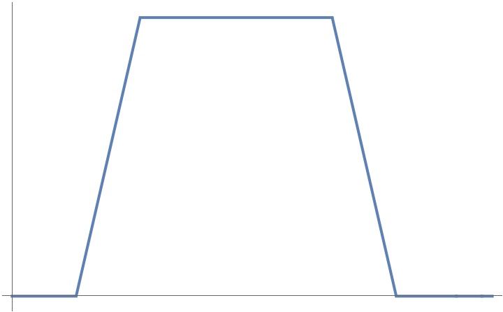
Once again, we would like to examine our system’s behavior in response to a force that is switched on for a period of time and then switched off. We will use a ‘top hat’ function like before, which consists of a ramp up, a constant period, and then a ramp back down to zero.

A spring-mass-damper system is subjected to a force given by the graph shown below.

This function can be specified in MATLAB using

function output = f1(t)
    % Builds a 'hat' from t = 2 to t = 12
    % using ramp functions.
    output = + heaviside(t-2).*5.*(t-2) + ...
             - heaviside(t-4).*5.*(t-4) + ...
             - heaviside(t-10).*5.*(t-10) + ...
             + heaviside(t-12).*5.*(t-12);
end

The differential equation can be implemented in MATLAB using

function dydt = rhs1(t,y,m)
% Define the right-hand side function of differential equation. It takes as
% input the value of m, which is a parameter we will change, in addition to
% the usual "t" and "y", where "y" is the state variable.
    b = 2; k = 4;

    x = y(1);
    xdot = y(2);

    dy1dt = xdot;
    dy2dt = (-b*xdot - k*x + f1(t))/m;

    dydt= [dy1dt;dy2dt];
end

Use the following starter code to investigate three values of \(m\) that show qualitatively different kinds of behaviorss. Describe how the behaviors you see are qualitatively different from each other.

% Define a time domain with lots of values
N     = 1000;
tvals = linspace(0,40,N);

% Call ode45 with initial conditions of zero using various values for m.
[t1,x1] = ode45(@(t,x) rhs1(t,x,1), tvals, [0;0]);

% Plot response 
clf;
yyaxis right;
plot(tvals,f1(tvals),'--',"LineWidth",1,'Color',"black");  hold on;
ylabel("Applied force f(t)")
yyaxis left;
plot(tvals,x1(:,1),'-',"LineWidth",2,"Color","blue"); hold on;
ylabel("Response x(t)")

% Make it pretty
set(gca,"FontSize",14);
pbaspect([3,1,1]);
xlabel("Time");

TipSolution

We make use of the following code.

% Define a time domain with lots of values
N     = 1000;
tvals = linspace(0,40,N);

mvals = [0.1,2,10];

% Call ode45 with initial conditions of zero using various values for m.
[t1,x1] = ode45(@(t,x) rhs1(t,x,mvals(1)), tvals, [0;0]);
[t2,x2] = ode45(@(t,x) rhs1(t,x,mvals(2)), tvals, [0;0]);
[t3,x3] = ode45(@(t,x) rhs1(t,x,mvals(3)), tvals, [0;0]);

% Plot response 
clf;
yyaxis right;
plot(tvals,f1(tvals),'--',"LineWidth",1,'Color',"black");  hold on;
ylabel("Applied force f(t)",'Color','black')
yyaxis left;
plot(tvals,x1(:,1),'-',"LineWidth",2,"Color","blue"); hold on;
plot(tvals,x2(:,1),'-',"LineWidth",2,"Color","cyan");
plot(tvals,x3(:,1),'-',"LineWidth",2,"Color","magenta");
legend("m = 0.1","m = 2", "m = 10");
ylabel("Response x(t)");
grid on;
grid minor;


% Make it pretty
set(gca,"FontName","EB Garammond","FontSize",16);
pbaspect([3,1,1]);
xlabel("Time");

% Save to file
saveas(gcf,"hat-response-sol.png");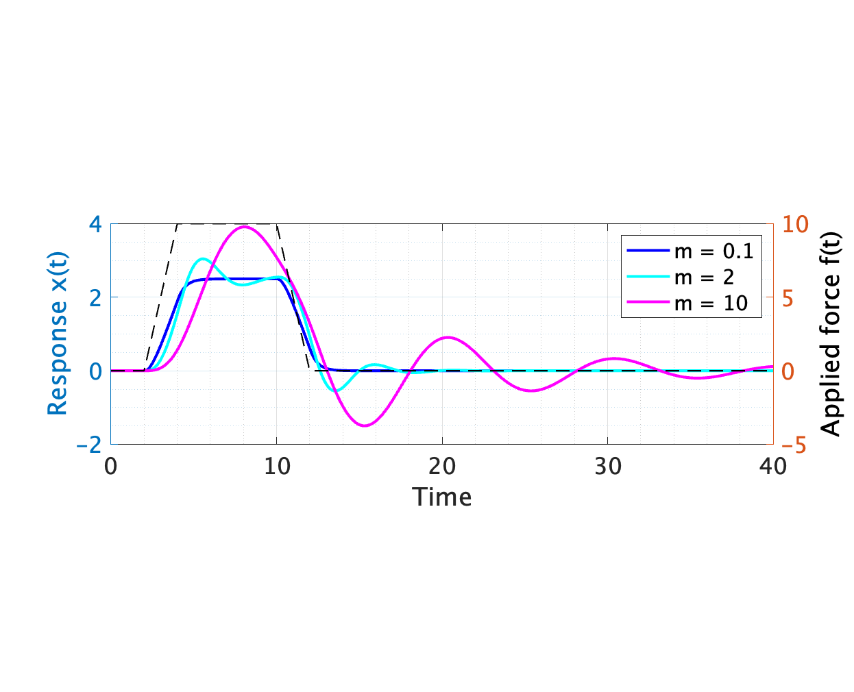

We see that when a small value of \(m=0.1\) is chosen, the response looks broadly similar to the applied force. There is not much ‘oscillation’ and things seem to smoothly flow from a ‘low’ state to a ‘high’ state and back.

When an intermediate value of \(m=2\) is chosen, the response is broadly similar, but this time with oscillations. It seems like the oscillations will die out if given enough time, but because the input is not ‘switched on’ for too long, the response doesn’t seem to have enough time to settle down.

When a large value of \(m=10\) is chosen, the system very much doesn’t seem to have enough of a chance to settle at any particular value and seems to be wildly going back and forth. It hardly seems to be following the input at all, but perhaps if given a very long time it will.

4 RLC Circuits

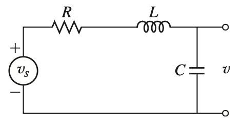
For the RLC circuit shown, it is known that the governing equation for the voltage across the capacitor is \[LC \ddot{v} + RC \dot{v} + v = v_s. \tag{6}\] When there is no input voltage and just a free response, what is the

1. Undamped natural frequency,
2. Damping ratio, and
3. Damped natural frequency

for the system? Give your answers in terms of \(R\), \(L\) and \(C\).

TipSolution

Let’s write the RLC equation and the spring-mass-damper equation in parallel with each other. We have \[ \begin{aligned} LC \ddot{v} + RC \dot{v} + v &= v_s \\ m \ddot{x} + b \dot{x} + k x &= f \end{aligned} \]

Quantity	Mechanical	Circuit
‘Mass’	\(m\)	\(LC\)
‘Damping’	\(b\)	\(RC\)
‘Spring Constant’	\(k\)	\(1\)

If we draw an analogy with the spring-mass-damper systems we’ve been looking at so far, we find that the undamped natural frequency should be ‘\(\sqrt{k/m}\)’, except that ‘\(k\)’ is equal to unity in Equation 6 and ‘\(m\)’ is equal to \(LC\) in Equation 6. Therefore, the undamped natural frequency is \[\omega_n = \sqrt{1/LC} = \boxed{(LC)^{-1/2}}\]

Similarly, the damping ratio in this system is ‘\(b/\sqrt{4mk}\)’ but \(k=1\), \(m=LC\) and \(b=RC\). So, drawing on the definition of the damping ratio \(\zeta\), we can write \[\zeta = \frac{RC}{\sqrt{4 LC}} = \boxed{\frac{1}{2} R C^{1/2} L^{-1/2}}\]

To determine the time constant, we can either use the definition \(1/(\zeta \omega_n)\) from lecture 14 or notice that the time constant is the inverse of the absolute value of the real part of the roots of the characteristic polynomial. The real part of the roots of the characteristic polynomial is \[-\frac{b}{2m}\] for the spring-mass-damper system, so by analogy we can write that the time constant is the inverse of \[ \frac{RC}{2 LC} = \frac{R}{2L},\] i.e. the time constant is \[\boxed{\frac{2L}{R}}\]