Lecture 23
E12 Linear Physical Systems Analysis
Plan for week 14
Comprehensive Final Assigment in class on Thursday to synthesize everything we have learned
No HW will be assigned on week 14
Tuesday:
- Instructor analyzes an electrical system on board
Thursday:
- You will analyze a mechanical system in class and turn in your work, including some/all of:
- State variables
- Differential Equation
- Laplace Transform
- Block Diagram
- Transfer Function
- Free Response
- Step Response
- Impulse Response
- Frequency Response
- Bode Plots
Input-Output Equations
In Lecture 12 we saw that the governing differential equations for linear physical systems can be written in the following form:
\[\dot{\boldsymbol{x}} = \boldsymbol{A} \boldsymbol{x} + \boldsymbol{B} \boldsymbol{u}\]
- \(\boldsymbol{x}\) is the state vector (\(n \times 1\))
- \(\boldsymbol{A}\) is the system matrix (\(n \times n\))
- \(\boldsymbol{B}\) is the input control matrix (\(n \times m\))
- \(\boldsymbol{u}\) is the input vector (\(m \times 1\))
\[{\boldsymbol{y}} = \boldsymbol{C} \boldsymbol{x} + \boldsymbol{D} \boldsymbol{u}\]
- \(\boldsymbol{y}\) is the output vector (\(p \times 1\))
- \(\boldsymbol{C}\) is the state output matrix (\(p \times n\))
- \(\boldsymbol{D}\) is the control output matrix (\(p \times m\))
Linear Input-Output Equations & State Variables
\[\dot{\boldsymbol{x}} = \boldsymbol{A} \boldsymbol{x} + \boldsymbol{B} \boldsymbol{u} \tag{1}\]
\[{\boldsymbol{y}} = \boldsymbol{C} \boldsymbol{x} + \boldsymbol{D} \boldsymbol{u} \tag{2}\]
Equation 1 is a differential equation for the state variables.
- The (rate of change of) state variables depends on (1) a linear combination of the state variables themselves, and (2) a linear combination of the input variables.
Equation 2 is an algebraic equation for the output variables.
- The output variables depend on (1) a linear combination of the state variables and (2) a linear combination of the input variables.
- If the output variables we want are the state variables, then \(\boldsymbol{C}\) is the identity matrix \(\boldsymbol{C} = \boldsymbol{1}\) and \(\boldsymbol{D} = \boldsymbol{0}\).
Side note: Nonlinear equations
\[\dot{\boldsymbol{x}} = \boldsymbol{A} \boldsymbol{x} + \boldsymbol{B} \boldsymbol{u}\]
- If \(\dot{\boldsymbol{x}} = ...\) is a nonlinear function of \(\boldsymbol{x}\) or of \(\boldsymbol{u}\),
- the above equation cannot be written.
- the differential equation can still be numerically solved using
ode45orsolve_ivp. - Cannot use the Laplace Transform
\[{\boldsymbol{y}} = \boldsymbol{C} \boldsymbol{x} + \boldsymbol{D} \boldsymbol{u}\]
- If \({\boldsymbol{y}} = ...\) is a nonlinear function of \(\boldsymbol{x}\) or of \(\boldsymbol{u}\),
- the above equation cannot be written.
- we can still use the nonlinear equation to obtain required outputs.
Multiple-Input, Multiple-Output systems
There are multiple options for how to write down the equations of a system. Let’s look at two.
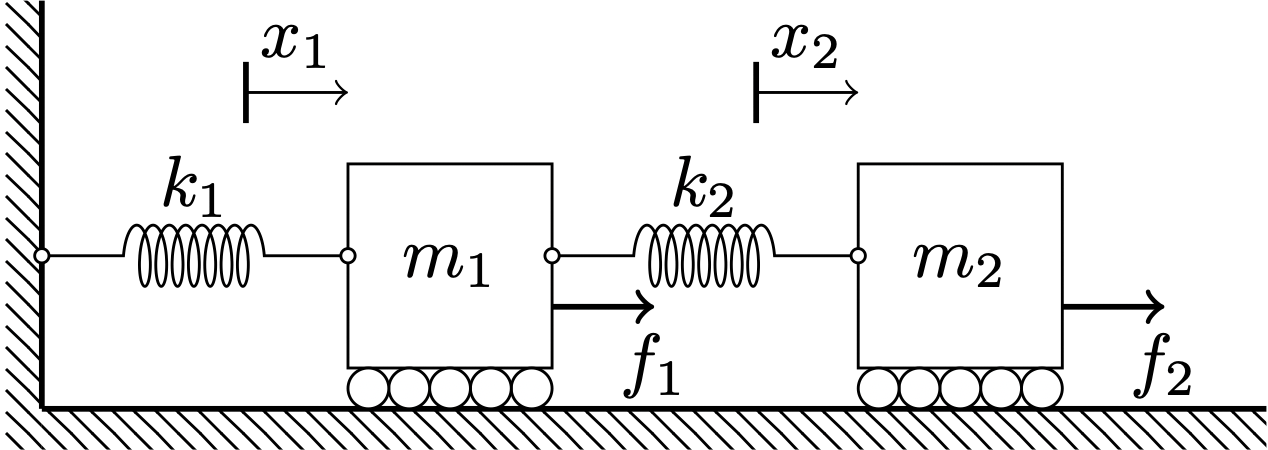
- Four state variables: \(x_1\), \(\dot{x}_1\), \(x_2\), \(\dot{x}_2\).
- Two inputs: \(f_1(t)\) and \(f_2(t)\).
- We are interested in three outputs:
- The position of the first mass \(x_1\)
- The distance between the two masses, \(x_2-x_1\)
- The total momentum of the system, \(m_1 \dot{x}_1 + m_2 \dot{x}_2\)
- Four state variables: \(x_1\), \(\dot{x}_1\), \(x_2-x_1\), \(\dot{x}_2\).
- Two inputs: \(f_1(t)\) and \(f_2(t)\).
- We are interested in three outputs:
- The position of the first mass \(x_1\)
- The position of the second mass, \(x_2\)
- The total potential elastic energy of the system, \(\frac{1}{2}k {x_1}^2 + \frac{1}{2} k x_2^2\)
Checking the validity of equations
\[ \begin{aligned} \dot{\boldsymbol{x}} &= \boldsymbol{A} \boldsymbol{x} + \boldsymbol{B} \boldsymbol{u} \\ {\boldsymbol{y}} &= \boldsymbol{C} \boldsymbol{x} + \boldsymbol{D} \boldsymbol{u} \end{aligned} \]
- The number of state variables should equal the number of energy-storing elements
- The output variables should be a linear combination of the input variables and the state variables.
- There are no restrictions on the number of input variables and output variables.
Note:
- Multiplying a matrix with a matrix is the same thing as a dot product
- A ‘(column) vector’ is the same as a ‘matrix with with 1 column’
- To correctly multiply \(A B\), a.k.a. \(A \cdot B\), the number of columns of \(A\) must equal the number of rows of \(B\)
- Matrix multiplication is not commutative, \(A \cdot B \neq B \cdot A\)
Constructing the input control matrix
\[ \frac{d}{dt} \begin{bmatrix} x_1 \\ \dot{x}_1 \\ x_2 \\ \dot{x}_2 \end{bmatrix} = \begin{bmatrix} 0 & 1 & 0 & 0 \\ -(k_1+k_2)/m_1 & 0 & k_2/m_1 & 0 \\ 0 & 0 & 0 & 1 \\ k_2/m_2 & 0 & -k_2/m_2 & 0 \end{bmatrix} \begin{bmatrix} x_1 \\ \dot{x}_1 \\ x_2 \\ \dot{x}_2 \end{bmatrix} + {\color{red}{\begin{bmatrix} 0 \\ f_1/m_1 \\ 0 \\ f_2/m_2 \end{bmatrix}}} \]
We can re-write the equations of this system in the form \[\dot{\boldsymbol{x}} = \boldsymbol{A} \boldsymbol{x} + \boldsymbol{B} \boldsymbol{u}\]
where \(\boldsymbol{u}\) is a vector of inputs. Here, \(\boldsymbol{u} = \begin{bmatrix} f_1 \\ f_2 \end{bmatrix}\)
to find \(\boldsymbol{B}\) we construct a matrix of size \(n \times m\)
- here, \(n\) is the number of state variables and \(m\) the number of inputs.
\[ \underbrace{{\color{magenta}{\begin{bmatrix} 0 & 0 \\ 1/m_1 & 0 \\ 0 & 0 \\ 0 & 1/m_2 \end{bmatrix}}}}_{\boldsymbol{\displaystyle B}} \begin{bmatrix} f_1 \\ f_2 \end{bmatrix} = {\color{red}{\begin{bmatrix} 0 \\ f_1/m_1 \\ 0 \\ f_2/m_2 \end{bmatrix}}} \]
Constructing the (linear) output equations
We are interested in three specific outputs:
- The position of the first mass \(x_1\)
- The distance between the two masses, \(x_2-x_1\)
- The total momentum of the system, \(m_1 \dot{x}_1 + m_2 \dot{x}_2\)
- To construct the output equation \[{\boldsymbol{y}} = \boldsymbol{C} \boldsymbol{x} + \boldsymbol{D} \boldsymbol{u}\]
- we need to express the output variables of interest (\(\boldsymbol{y}\)) as a linear combination of
- the state variables (\(\boldsymbol{x}\)) and
- the input variables (\(\boldsymbol{u}\)).
- Let \(y_1 = x_1\)
- Let \(y_2 = x_2-x_1\)
- and \(y_3 = m_1 \dot{x}_1 + m_2 \dot{x}_2\)
- So we have \[\boldsymbol{C} = \begin{bmatrix} +1 & 0 & 0 & 0 \\ -1 & 0 & +1 & 0 \\ 0 & m_1 & 0 & m_2 \end{bmatrix}, \]
- multiplying \[ \boldsymbol{x} = \begin{bmatrix} x_1 \\ \dot{x}_1 \\ \dot{x}_2 \\ \dot{x}_2 \end{bmatrix} \]
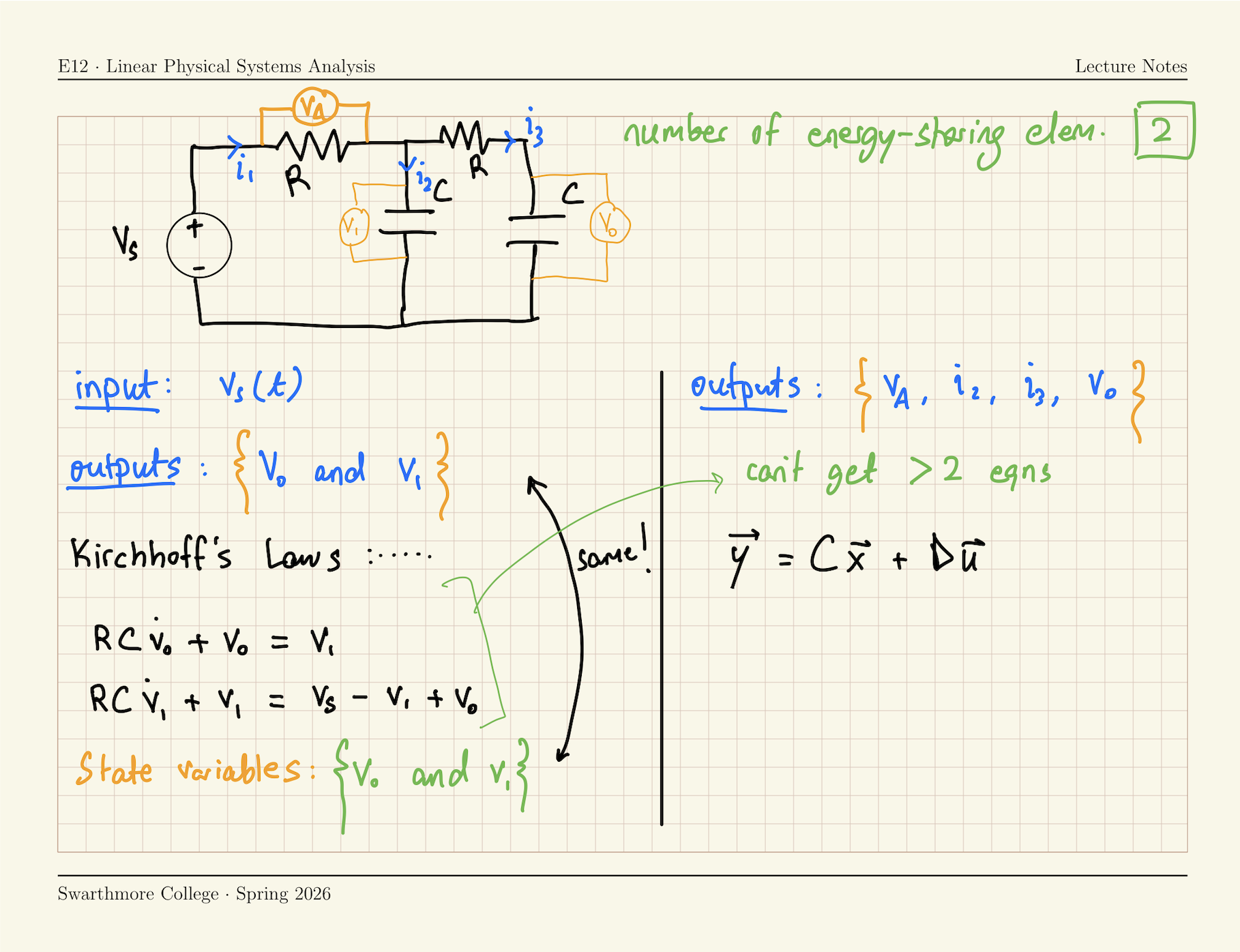
Two outputs in a circuit