Problem Set 3
ENGR 12, Spring 2026.
| Due Date | Thu, Feb 12, 2026 |
| Turn in link | Gradescope |
| URL | emadmasroor.github.io/E12-S26/Homework/HW3 |
Points Distribution
For this assignment, the problems are unequally weighted. More weightage has been assigned to problems that have several parts. Scores will be assigned on a 3-2-1-0 scale. For problems with 3 points available, the possible scores are 3,2,1 and 0. For problems with 6 points available, the possible scores are 6,4,2 and 0.
| Problem | Part | % Weightage | Points |
|---|---|---|---|
| Problem 1 | 1.1 | 10 | 3 |
| 1.2 | 10 | 3 | |
| 1.3 | 20 | 6 | |
| 1.4 | 20 | 6 | |
| Problem 2 | 2.1 | 20 | 6 |
| 2.2 | 10 | 3 | |
| 2.3 | 10 | 3 |
1 Laplace Transform
1.1 Computing the integral explicitly without using the table
Using the definition of the Laplace Transform given in lecture, determine the Laplace Transform of the function \(x(t) = c t\) by integration. The result should be a function of \(s\) and \(c\).
1.2 Deriving expressions for the Laplace Transform using the table
This question asks for a derivation of a result that you already know from the table. Thus, you cannot simply copy the result from the table; you have to ‘prove’ it mathematically.
- \(\displaystyle \mathcal{L}\left[ e^{-at}\right] = \frac{1}{s+a} ,\) i.e., the Laplace transform of \(e^{-at}\) is \(1/(s+a)\).
- The Linearity Property holds.
- Euler’s formula holds, i.e., \(\displaystyle e^{i x} = \cos x + i \sin x\)
and the usual rules of complex algebra.
Show that the Laplace Transform of the function \(\sin \omega t\) is \(\displaystyle \frac{\omega}{s^2+\omega^2}\).
Start by writing out the trigonometric terms \(\cos \omega t\) and \(\sin \omega t\) as sums of exponential terms.
1.3 Computing Laplace transforms using the table
Compute the Laplace Transform of the following functions and give your answers as rational functions of the frequency \(s\). For each answer, write down the order of the numerator polynomial and the order of the denominator polynomial.
Use the table of Laplace transform pairs.
- \(f(t) = 1 + 2t - 3t^3\)
- \(f(t) = \cos \omega_1 t + \cos \omega_2 t\)
- \(f(t) = t^3 e^{-5t}\)
1.4 Computing Inverse Laplace Transforms using the table
For each of the following functions \(F(s)\), find \(f(t)\), the result of applying the inverse Laplace Transform \(\mathcal{L}^{-1}\) to \(F\).
Use the table of Laplace transform pairs.
Recall that if a polynomial equals zero at two complex roots \(z = a \pm i b\) when that polynomial can be written as \[(s+a)^2+b^2.\]
- \[F(s) = \frac{3s+1}{s(s+4)}\]
- \[F(s) = \frac{s}{s^2+3} + \frac{\sqrt{3}}{s^2+3}\]
- \[F(s) = \frac{2}{s^2+3s+4}\]
- \[F(s) = \frac{1}{(s+4)(s-4)}\]
2 The Free and Forced Response
2.1 The Free and Forced Response in frequency domain
Consider an RC circuit with a variable voltage source. The capacitor initially has \(1.5\) volts across it.

For each of the following cases, write down a mathematical expression for the free response and a mathematical expression for the forced response of the capacitor in the frequency domain.
Think of the capacitor voltage as the output of your system, and the time-varying voltage source as the input. The word ‘response’ refers to “the way the output responds to the input”.
Do not simplify your expressions using Partial Fractions for this question. Leave your answers as rational functions.
- \(v_s(t) = 0\) V, a constant equal to zero.
- \(v_s(t) = 5.0\) V, a nonzero constant.
- \(v_s(t) = 2t\) V, a ramp input.
- \(v_s(t) = 5 \cos 2t\) V, a sinusoidally-varying input.
2.2 Mathematical Expressions for the free and forced response in frequency and time domains
For this problem, consider a system subjected to a ramp input, \[\dot{x} + a x = f(t) = c t \tag{1}\] where \(x(t)\) is the output we care about, and the input is a simple linear function of time. Let the initial condition be \(x(0) = x_0\)
Using a procedure similar to the one carried out in class for a constant input, determine the free response and forced response in terms of \(a\) and \(c\), in both the frequency domain and in the time domain.
To solve this problem, you will need to break apart a rational function into a sum of partial fractions.
2.3 Application to a mechanical system.
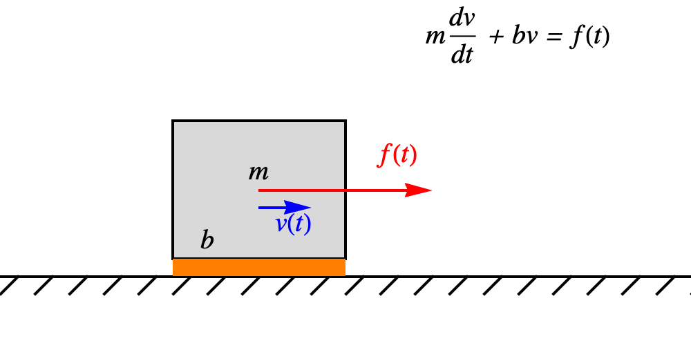
(In some suitable and correct system of units,) consider an object of mass \(m = 1\) with friction coefficient \(b = 3\) subjected to a ramped force \(f(t) = ct\) where \(c=2\). The object was initially moving at a speed of \(1\).
Make a plot similar to the one in lecture showing the free response, forced response, and total response of the object’s speed \(v(t)\) to the applied force \(f(t)\). You will make three line plots, and they should be on the same set of axes. Choose an appropriate range for the horizontal and vertical axes such that the interesting dynamics are illustrated clearly.