flowchart LR
  E[Input] --> F[System] --> G[Output]
Lecture 1
E12 Linear Physical Systems Analysis
Welcome to E12
- Prof. Emad Masroor
- B.S. Mechanical Engineering, Cornell University 2017
- Ph.D. Engineering Mechanics, Virginia Tech 2023
- Visiting Assistant Professor at Swarthmore College since fall 2023
- Research interests broadly in Fluid Dynamics:
- theory, experiment, computation
- Energy harvesting from wind and water
- Biological locomotion in fluids (swimming/flying)
Teaching Team
| Name | Role |
|---|---|
| Emad Masroor | Lecture Instructor |
| Will Johnson | Laboratory Instructor |
| Kenny Relovsky | Course Wizard |
| Madeline Mountcastle | Course Wizard |
| Bella Thoen | Course Wizard |
| Tanvir Islam | Course Wizard |
| Miles Fleisher | Lab Wizard |
| Nick Fettig | Lab Wizard |
| Aubree Daugherty | Grader |
| Ryder Maston | Grader |
| Owen Hoffman | Grader |
| Howard Wang | Grader |
| Julian Courtney-Bacher | Grader |
Introductions
This class is typically taken by Engineering majors in their sophomore year. If this does not describe you, please include your major and year (junior, senior, etc.) in your introduction.
- Name
- Hometown
- Last T.V. show you watched
- Agree or disagree: “B is a good grade”
Homework Zero
- A homework assignment is due this Thursday at midnight.
- If you need help with it, don’t hesitate to ask for it!
What is E12 all about?
Linear Physical Systems Analysis
You have already learned how to analyze two types of physical systems
- Mechanical (E6)
- Electrical (E11)
This underlying mathematics and techniques of analysis are actually shared across various types of physical systems.
Let’s look at each term in turn.
Linear Physical Systems Analysis
- Familiar physics from E6 and E11
- Circuits and mechanical systems
- New in mechanics: motion (Newtonian mechanics)
- “New” physics will be introduced, but the focus of this class is not physics
Linear Physical Systems Analysis
- For now, let’s define a system as a black box that connects inputs to outputs.
- For a system to make sense and to be a reasonable model of (most) physical processes, it should always give the same output for the same input.
- Let’s set aside for the moment any uncertainty, randomness, chaos, etc.
- But wait, we already have a math concept for this! A mathematical object that takes in inputs and gives you outputs
- A function \(y = f(x)\)
- Our functions must be one-to-one, a.k.a. injective.
Linear Physical Systems Analysis
- “Resolution into simpler elements by analysing (opp. synthesis)”
- Breaking something down into simpler constituent pieces
Linear Physical Systems Analysis
- Let’s think about the word linear. It is an adjective derived from the noun line. So linearity has something to do with lines.
- What are some properties of lines?
- They go off to infinity in both directions
- They have a constant slope
- All possible lines in two dimensions are given by two numbers:
- \(y = mx + b\)
- \(m\) and \(b\)
- More to come …
E12 Class Organization & Logistics
Find the syllabus on the class website.
- HW is due on Thursdays at midnight
- HW Zero is due this Thursday Jan 22, graded on completion.
- Weekly problem-solving session Monday evening
- Wizard sessions Wednesday evening
- One midterm exam the week after spring break, Thu 03/19 7 PM evening
- One final exam (cumulative)
Consult syllabus for details.
Textbooks
Palm (3rd or 4th ed.) required; Close Frederick & Newell optional
Linear vs. Nonlinear Equations
- Consider the following equations:
\[2a + 3b = 0 \tag{1}\] \[2ab + 3 = 0 \tag{2}\]
- Guess two solutions for each of these equations independently — two solutions for Equation 1, and two solutions for Equation 2
Separately for each equation, do the following tasks:
Task 1
- Choose one of your two solutions.
- Multiply this solution by 2
- Check if the resulting values of \(a\) and \(b\) are solutions to the equation.
Task 2
- Add the two solutions to each other
- You now have a new value of \(a\) and \(b\).
- Check if the new values of \(a\) and \(b\) are solutions to the equation.
Linear vs. Nonlinear equations
Linear vs. Nonlinear equations
\[2a + 3b = 0\] \[2ab + 3 = 0\]
From our exercise, it appears that:
- An equation is linear if a solution to that equation, when multiplied by a constant scalar, is also a solution to the same equation.
- If this property does not hold, then the equation is non-linear
- An equation is linear if one solution to that equation, when added to a different solution to that equation, gives a new solution to the original equation.
- If this property does not hold, then the equation is non-linear
This heuristic will later be further refined and qualified.
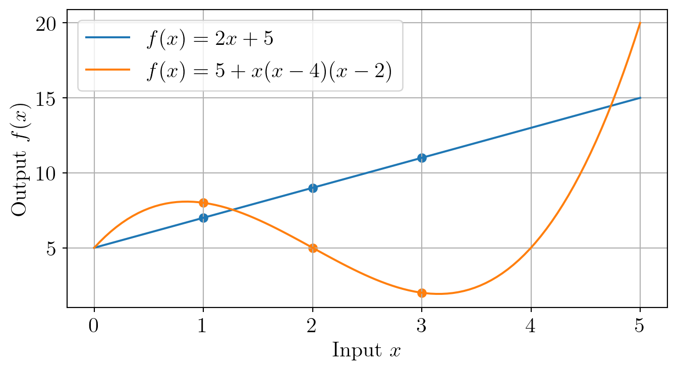
A linear vs. nonlinear function
Consider the following two functions.
Code
import numpy as np
import matplotlib.pyplot as plt
from matplotlib import rc

def f1(x): # a linear function
  return 2*x+5

def f2(x): # a non-linear function
  return 5 + (x - 4)*(x)*(x - 2)

# Create an 'x axis' with 100 points from 0 to 5
x_vals = np.linspace(0,5,100)

# Size the figure
plot1 = plt.figure(figsize=(8, 6))

# Font stuff
plt.rcParams.update({
    "text.usetex": True,
    "font.family": "serif",
    "font.serif": ['Computer Modern Roman'],
    "font.size": 16
})
# ----

plt.plot(x_vals,f1(x_vals),label="$f(x) = 2x + 5$")
plt.plot(x_vals,f2(x_vals),label="$f(x) = 5 + x(x-4)(x-2)$")
plt.xlabel("Input $x$",fontsize=20)
plt.ylabel("Output $f(x)$",fontsize=20)
plt.legend()
plt.grid()
plt.show()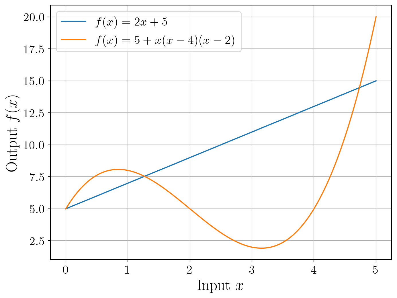
Both seem predictable …
| 1.0 | 2.0 | 3.0 | 4.0 | 5.0 | |
|---|---|---|---|---|---|
| System 1 (Linear) | 7 | 9 | 11 | ||
| System 2 (Nonlinear) | 8 | 5 | 2 |
- It seems that the outputs are predicted well by the inputs.
- In particular, it seems that how you change the input changes the output in a regular way.
- In system 1, you get an increase of 2 if you dial up the output by 1
- In system 2, you get a decrease of 3 if you dial up the output by 1
But nonlinear systems run into trouble
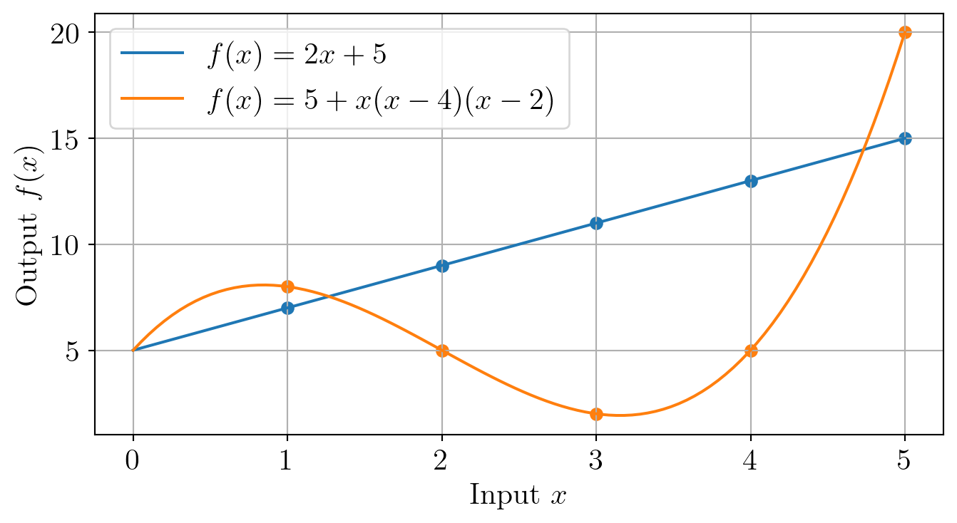
| 1.0 | 2.0 | 3.0 | 4.0 | 5.0 | |
|---|---|---|---|---|---|
| System 1 (Linear) | 7 | 9 | 11 | 13 | 15 |
| System 2 (Nonlinear) | 8 | 5 | 2 | 5 | 20 |
However, this does not last for system 2; the predictability breaks down.
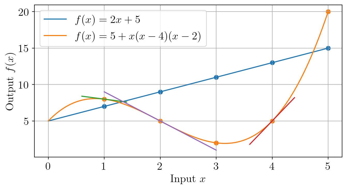
Linearizing a nonlinear system
The input of a certain system is \(x\) and the output is \(f(x)\), and the inputs and outputs are related as
\[f(x) = x^2 - 3 x + 1\]
TipQuickly plotting functions
You should be familiar with at least one technique for quickly plotting a function using a calculator or computer. I like Mathematica for this purpose. You are recommended to use a program that can easily export plots as images.
We are looking for a linear approximation to \(f(x)\), i.e., \(f^*(x) \approx f(x)\) where \(f^*(x)\) is linear in \(x\).
Task 1: Write down a linear model \(f^*(x)\) for this system that is applicable everywhere
Task 2: Write down a linear model \(f^*(x)\) for this system that is applicable:
- near \(x=0\)
- near \(x=3\)
We can linearize nonlinear systems for a while
In the neighborhood of a point, it’s possible to make linear approximations to \(f(x)\) using the derivative \(f'(x)\).
Homework 1 will have a problem based on this.