Problem Set 6 Solutions
ENGR 12, Spring 2026.
Solutions
1 A coupled first-order system
In HW 1, we looked at the system of equations governing the (somewhat idealized) motion of one box on top of another box as shown in the diagram below.

The governing equations for the system shown schematically above are
\[ \begin{aligned} m_1 \dot{v}_1 &+ b_1 v_1 =0 \\ m_2 \dot{v}_2 &+ b_2 (v_2-v_1) = 0 \end{aligned} \tag{1}\]
1.1 Deriving the equations
Express Equation 1 in the form of Equation 3, using an appropriate set of state variables.
Let’s define the state variables to be the two momenta: \(m_1 v_1\) and \(m_2 v_2\). (It would be okay to use \(v_1\) and \(v_2\), too) In terms of these equations, we can write the governing equations to be
\[ \frac{d}{dt} \begin{bmatrix} m_1 v_1 \\ m_2 v_2 \end{bmatrix} = \begin{bmatrix} m_1 \dot{v}_1 \\ m_2 \dot{v}_2 \end{bmatrix} = \begin{bmatrix} -b_1 v_1 \\ b_2 v_1 - b_2 v_2 \end{bmatrix} \] We can then write this equation as a matrix multiplying the state vector as follows: \[ \frac{d}{dt} \begin{bmatrix} m_1 v_1 \\ m_2 v_2 \end{bmatrix} = \begin{bmatrix} -b_1/m_1 & 0 \\ b_2/m_2 & -b_2/m_2 \end{bmatrix} \begin{bmatrix} m_1 v_1 \\ m_2 v_2 \end{bmatrix} \]
1.2 Solving in MATLAB
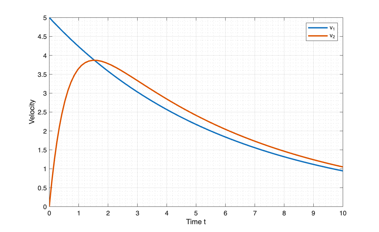
Solve these equations using ode45, starting from the skeleton code given below. Use parameter values \(m_1 = 30, m_2 = 3, b_1 = b_2 = 5\), and initial conditions \(v_1 = 5\) and \(v_2 = 0\) at \(t=0\). Continue your plot up to time \(t=10\).
You need not use exactly the same state variables that you chose in the previous part; use whatever set of state variables seems convenient and intuitive.
The given code has a serious mistake, but it should be pretty straightforward to fix.
% Define the system of ODEs
% y(1) = v1, y(2) = v2
function dvdt = odefun(t, y)
    % Parameters
    m1 = 30;
    m2 = 3;
    b1 = 5;
    b2 = 5;

    % Unpack
    v1 = y(1);
    v2 = y(2);

    % Define rhs of differential equations
    % m1*v1' + b1*v1 = 0  => v1' = -b1*v1 / m1
    % m2*v2' + b2*(v2 - v1) = 0 => v2' = -b2*(v2 - v1) / m2
    dvdt = [(-b1 * v1) / m1;
            0.5];
end

% Solve
% Initial conditions: v1(0) = 5, v2(0) = 0
[t, sol] = ode45(@odefun, [0, 10], [5; 0]);

% Extract results
v1 = sol(:,1);
v2 = sol(:,2);

% Create the plot
figure(1); clf;
plot(t, v1, t, v2); grid on; grid minor;
legend('v_1', 'v_2');
xlabel('Time t');
ylabel('Velocity');To solve this problem, we just need to fix a single line of code, highlighted in the comment below.
% Define the system of ODEs
% y(1) = v1, y(2) = v2
function dvdt = odefun(t, y)
    % Parameters
    m1 = 30;
    m2 = 3;
    b1 = 5;
    b2 = 5;

    % Unpack
    v1 = y(1);
    v2 = y(2);

    % Define rhs of differential equations
    % m1*v1' + b1*v1 = 0  => v1' = -b1*v1 / m1
    % m2*v2' + b2*(v2 - v1) = 0 => v2' = -b2*(v2 - v1) / m2
    dvdt = [(-b1 * v1) / m1;
            (-b2 * (v2 - v1)) / m2]; % <---- Correct -----|
end

% Solve
% Initial conditions: v1(0) = 5, v2(0) = 0
[t, sol] = ode45(@odefun, [0, 10], [5; 0]);

% Extract results
v1 = sol(:,1);
v2 = sol(:,2);

% Create the plot
figure(1); clf;
plot(t, v1, t, v2); grid on; grid minor;
legend('v_1', 'v_2');
xlabel('Time t');
ylabel('Velocity');
The end result is the figure below.
2 State-variable form and MATLAB
For each of the given systems of equations, complete the following tasks:
- Identify the \(n\) state variables
- Write the equations in the form \[\frac{d}{dt} \begin{bmatrix} y_1 \\ y_2 \\ \vdots \\ y_n \end{bmatrix} = \begin{bmatrix} f_1(y_1,y_2,...,y_n) \\ f_2(y_1,y_2,...,y_n) \\ \vdots \\ f_n(y_1,y_2,...,y_n) \end{bmatrix} + \begin{bmatrix} g_1(t) \\ g_2(t) \\ \vdots \\ g_n(t) \end{bmatrix} \tag{2}\]
- If possible, re-write the equations in the form \[\frac{d}{dt} \begin{bmatrix} y_1 \\ y_2 \\ \vdots \\ y_n \end{bmatrix} = \begin{bmatrix} a_{11} & a_{12} & \dots & a_{1n} \\ a_{21} & a_{22} & \dots & a_{2n} \\ & & \vdots & \\ a_{n1} & a_{n2} & \dots & a_{nn} \end{bmatrix} \begin{bmatrix} y_1 \\ y_2 \\ \vdots \\ y_n \end{bmatrix} + \begin{bmatrix} g_1(t) \\ g_2(t) \\ \vdots \\ g_n(t) \end{bmatrix} \tag{3}\]
- Write down the MATLAB (or Python) code that will successfully solve the initial value problem.
2.1
\[ \begin{aligned} \dot{x}_1 x_2 + 5 x_2 &= -3 x_1 x_2 - 2 x_2 t \\ \dot{x}_2 + 3x_1 &= 7 x_2 \end{aligned} \]
With initial conditions \(x_1(0) =1\) and \(x_2(0) = -3\). We are interested in the behavior of this system up to time \(t=5\).
Note that we must first divide through the first equation by \(x_2\), and the resulting constant term can be folded into either \(f_1\) or \(g_1\). We choose to fold it into \(g_1\) so that we can write \(f_1\) and \(f_2\) as a matrix times \([x_1, x_2]\)
- The state variables are \(x_1\) and \(x_2\).
- The state-variable equations are \[ \begin{aligned} \frac{d}{dt} \begin{bmatrix} x_1 \\ x_2 \end{bmatrix} &= \begin{bmatrix} f_1(x_1,x_2) \\ f_2(x_1,x_2) \end{bmatrix} + \begin{bmatrix} g_1(t) \\ g_2(t) \end{bmatrix} \\ &= \begin{bmatrix} -3x_1 \\ -3x_1 - 7 x_2 \end{bmatrix} + \begin{bmatrix} -5 -2t \\ 0 \end{bmatrix} \end{aligned} \]
- Emphasizing the linearity of the equations, we can write \[ \begin{aligned} \frac{d}{dt} \begin{bmatrix} x_1 \\ x_2 \end{bmatrix} &= \begin{bmatrix} -3 & 0 \\ -3 & -7 \end{bmatrix} \begin{bmatrix} x_1 \\ x_2 \end{bmatrix} + \begin{bmatrix} -5 -2t \\ 0 \end{bmatrix} \end{aligned} \]
- MATLAB code to solve this problem is given below.
function dxdt = rhs(t,x)
    % un-pack contents of y
    x1 = x(1); x2 = x(2);

    % Define what dx/dt is
    dx1dt = -3*x1 -5 - 2*t;
    dx2dt = -3*x1-7*x2;

    % Assemble contents of dx/dt into a column vector
    dxdt = [dx1dt;dx2dt];
end

% Use ode45 from t = 0 to t = 5. Initial conditions are
% x(0) = 1, x'(0) = -3
[t,ysol] = ode45(@rhs,[0,5],[1;-3]);

% Make plot
clf;
plot(t,ysol); % Plots both columns of 'ysol' in one go
legend("x1","x2","Location","east");

% Format plot nicely
set(0, 'DefaultLineLineWidth', 2);
title("Problem 1.1")
set(gca,"FontName","EB Garamond");
set(gca,"LineWidth",1);
xlabel("Time [seconds]");
set(gca,"FontSize",20);
grid on;

% Save it
saveas(gcf,"MATLABfig3.png")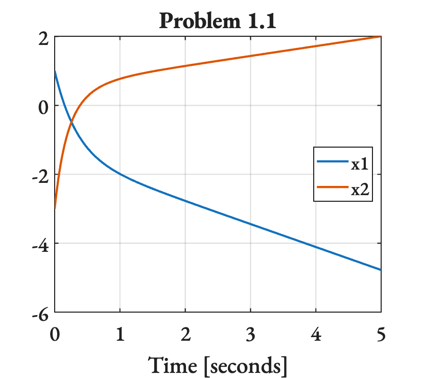
2.2
\[ \begin{aligned} 3\dot{x} + 5 y &= 2x - \dot{y} \\ 2\dot{y} - 7x &= 4y + \dot{x} \end{aligned} \]
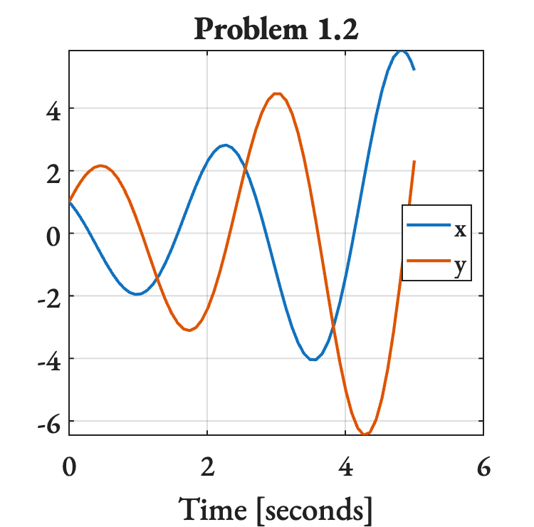
With initial conditions \(x(0) =1\) and \(y(0) = 1\). We are interested in the behavior of this system up to time \(t=5\).
- There are two state variables: \(x\) and \(y\).
- To put the equations in state-variable form, we must first manipulate the equations until we get a form where there is only one derivative in each equation. Using the substitutions \[\dot{y} = -3\dot{x} - 5 y + 2x, \quad \dot{x} = 2 \dot{y} - 7x - 4y,\] we can write \[ \begin{aligned} 3 \dot{x} + 5 y &= 2x - \dot{y} \\ 3(2 \dot{y} - 7x - 4y) + 5y &= 2x - \dot{y} \\ 7 \dot{y} - 21x - 12y +5y &= 2x \\ \dot{y} &= \frac{23}{7}x + y \end{aligned} \] and \[ \begin{aligned} \dot{x} &= 2 \dot{y} - 7x - 4y \\ &= 2 \left( \frac{23}{7}x + y \right) - 7x - 4y \\ \dot{x} &= -\frac{3}{7}x - 2y \end{aligned} \] Thus, the state-variable equations are \[ \frac{d}{dt} \begin{bmatrix} x \\ y \end{bmatrix} = \begin{bmatrix} -\frac{3}{7}x - 2y \\ \frac{23}{7}x + y \end{bmatrix} \]
- The linearity of the equations can be seen more clearly by putting them into the following form: \[ \frac{d}{dt} \begin{bmatrix} x \\ y \end{bmatrix} = \begin{bmatrix} -\frac{3}{7} & -2 \\ \frac{23}{7} & 1 \end{bmatrix} \begin{bmatrix} x \\ y \end{bmatrix} \]
- MATLAB code to solve this problem is given below.
function dzdt = rhs(t,z)
    % un-pack contents of z
    x = z(1); y = z(2);

    % Define what dz/dt is
    dxdt = -(3/7)*x - 2*y;
    dydt = (23/7)*x + y;

    % Assemble contents of dx/dt into a column vector
    dzdt = [dxdt;dydt];
end

% Use ode45 from t = 0 to t = 5. Initial conditions are
% x(0) = 1, x'(0) = 1
[t,ysol] = ode45(@rhs,[0,5],[1;1]);

% Make plot
clf;
plot(t,ysol); % Plots both columns of 'ysol' in one go
legend("x","y","Location","east");

% Format plot nicely
set(0, 'DefaultLineLineWidth', 2);
title("Problem 1.2")
set(gca,"FontName","EB Garamond");
set(gca,"LineWidth",1);
xlabel("Time [seconds]");
set(gca,"FontSize",20);
grid on;

% Save it
saveas(gcf,"MATLABfig4.png")
and the resulting figure is shown below.
2.3
\[ \begin{aligned} \dddot{x} &= -2\ddot{x} - 3 \dot{x} + 5 x - t \\ x(0) &= 1 \\ \dot{x}(0) &= -1 \\ \ddot{x}(0) &= 0 \end{aligned} \]
- There are three state variables: \(x\), \(\dot{x}\) and \(\ddot{x}\).
- To put this equation into state-variable form, we can simply write down \[ \begin{aligned} \frac{d}{dt} \begin{bmatrix} x \\ \dot{x} \\ \ddot{x} \end{bmatrix} = \begin{bmatrix} \dot{x} \\ \ddot{x} \\ -2\ddot{x} - 3 \dot{x} + 5 x - t \end{bmatrix} \end{aligned} \] and after this, we decide to call the state variables \(z_1\), \(z_2\) and \(z_3\). With this terminology, we can write \[ \begin{aligned} \frac{d}{dt} \begin{bmatrix} z_1 \\ z_2 \\ z_3 \end{bmatrix} = \begin{bmatrix} z_2 \\ z_3 \\ -2 z_3 - 3 z_2 + 5 z_1 - t \end{bmatrix} \end{aligned} \]
- To express the foregoing equation in a form that emphasizes linearity in the state variables, we can write \[ \begin{aligned} \frac{d}{dt} \begin{bmatrix} z_1 \\ z_2 \\ z_3 \end{bmatrix} = \begin{bmatrix}0 & 1 & 0 \\ 0 & 0 & 1 \\ 5 & -3 & -2 \end{bmatrix} \begin{bmatrix} z_1 \\ z_2 \\ z_3 \end{bmatrix} + \begin{bmatrix} 0 \\ 0 \\ -t \end{bmatrix} \end{aligned} \]
- This third-order system can be solved in MATLAB using the
ode45integrator using the following procedure.
function dzdt = rhs(t,z)
    % un-pack contents of z
    x       = z(1);
    dxdt    = z(2);
    d2xdt2  = z(3);

    % Define what d3x/dt3 is
    d3xdt3  = -2*d2xdt2-3*dxdt+5*x-t;

    % Assemble contents of dz/dt into a column vector
    dzdt = [dxdt;d2xdt2;d3xdt3];
end

% Use ode45 from t = 0 to t = 3. Initial conditions are
% x(0) = 1, x'(0) = -1, and x''(0) = 0
[t,ysol] = ode45(@rhs,[0,3],[1;-1;0]);

% Make plot
clf;
plot(t,ysol); % Plots both columns of 'ysol' in one go
legend("x","x'","x''","Location","north");

% Format plot nicely
set(0, 'DefaultLineLineWidth', 2);
title("Problem 1.3")
set(gca,"FontName","EB Garamond");
set(gca,"LineWidth",1);
xlabel("Time [seconds]");
set(gca,"FontSize",20);
grid on;

% Save it
saveas(gcf,"MATLABfig5.png")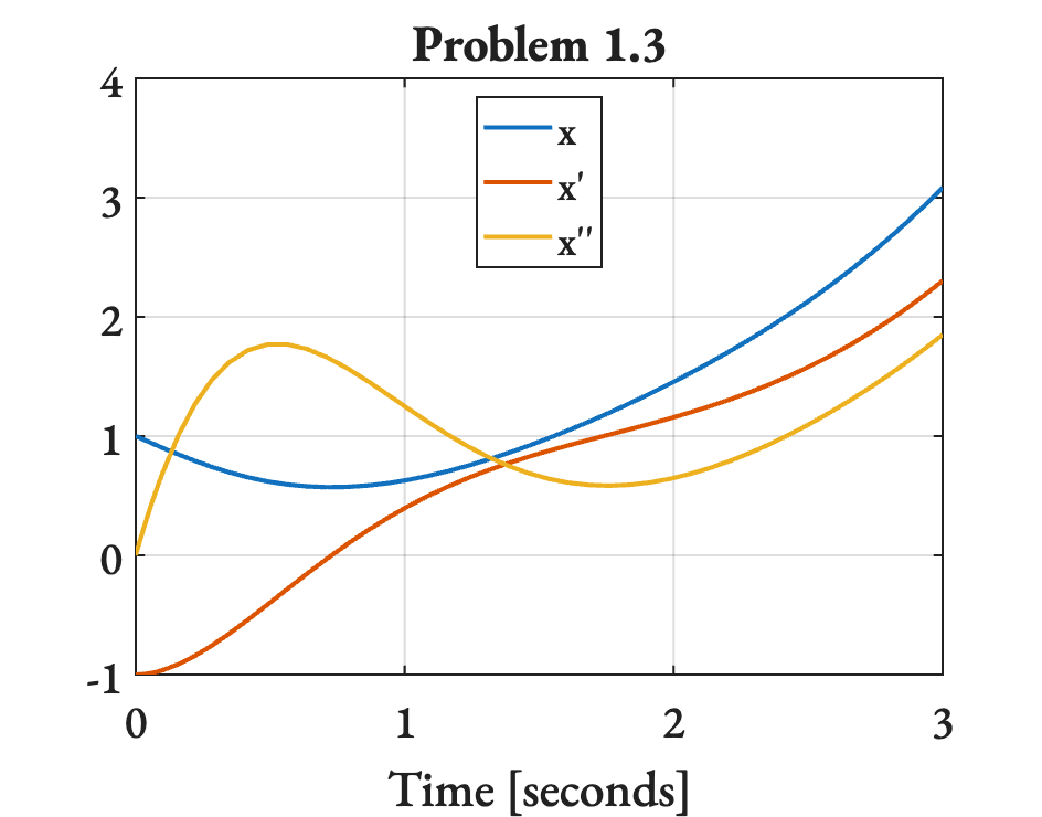
3 Choosing the right state variables
In class, we discussed the system shown below.

In this problem, please ignore \(f_1\) and \(f_2\). They are both equal to zero for now. Later, we will make use of these ‘input functions’ as well, but you’re off the hook for now!
3.1 Developing the equations
Write down the governing differential equations for this system in three forms:
- As two second-order differential equations for \(x_1(t)\) and \(x_2(t)\)
- As four first-order differential equations in state-variable form, arranged in the format of Equation 2. Name your four state variables \(y_1\), \(y_2\), \(y_3\) and \(y_4\).
- As three first-order differential equations in the state-variable form of Equation 2, using the following state variables: \[z_1 = \dot{x}_1, \quad z_2 = \dot{x}_2, \quad z_3 = x_2 - x_1\]
- By using free-body diagrams, it is possible to see that the governing equations for this system are \[ \begin{aligned} m_1 \ddot{x}_1 &= \phantom{-}k(x_2 - x_1) \\ m_2 \ddot{x}_2 &= -k(x_2-x_1) \end{aligned} \]
- It is straightforward to use the above equations to define four first-order equations. We have \[y_1 = x_1, \quad y_2 = \dot{x}_1, \quad y_3 = x_2, \quad y_4 \dot{x}_2\] and so the equations become \[ \begin{aligned} \dot{y}_1 &= y_2 \\ \dot{y}_2 &= \phantom{-}\frac{k}{m_1}(y_3 - y_1) + f_1 \\ \dot{y}_3 &= y_4 \\ \dot{y}_4 &= -\frac{k}{m_2}(y_3 - y_1) + f_2 \end{aligned} \tag{4}\]
- Using the definitions given in the question, the governing equations can be written as \[ \begin{aligned} \dot{z}_1 &= \left( \phantom{-}\frac{k}{m_1} \right) z_3 \\ \dot{z}_2 &= \left( -\frac{k}{m_2} \right) z_3 \\ \dot{z}_3 &= z_2 - z_1 \end{aligned} \tag{5}\]
3.2 Solving the equations
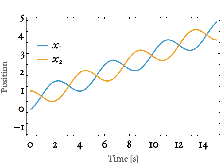
By modifying the MATLAB code provided on the website, write a program that simulates what happens to this system and plot your result. Your plot should show three quantities on the same set of axes, and should go from \(t=0\) to \(t=15\). The three quantities are \(z_1\), \(z_2\) and \(z_3\) as defined above. Use the following values for the parameters: \(m_1 = m_2 = k = 1\). The initial conditions are as follows:
- Mass 1 is initially moving at a velocity of \(0.5\) to the right
- Mass 2 is initially at rest
- The distance between Mass 2 and Mass 1, i.e., \(x_2-x_1\), is initially equal to \(1.0\)
You can ignore units for the purpose of this problem. Note that the position of the two masses with parameters and initial conditions as given above is given by the following graph.
The figure above can be produced using the following code.
% Define the system of ODEs
% y(1) = x1, y(2) = dx1/dt, y(3) = x2, y(4) = dx2/dt
function dydt = odefun(t,y)
    % Parameters
    m1 = 1; m2 = 1; k = 1;

    % Unpack
    x1      = y(1);
    x1dot   = y(2);
    x2      = y(3);
    x2dot   = y(4);

    % Define rhs of diff. eq.
    dydt = [x1dot;
            k*(x2-x1)/m1;
            x2dot;
            -k*(x2-x1)/m2];
end

% Solve for t = 0 to t= 15, with initial conditions
% on x1 = 0, x2 = 1, x1' = 0.5, x2' = 0
[t, sol] = ode45(@odefun, [0,15], [0; 0.5; 1; 0]);

% Extract results for plotting
x1 = sol(:,1);
x2 = sol(:,3);

% Create the plot
figure(1); clf;
hold on;
plot(t, x1, 'r-', 'LineWidth', 0.5);      % x1
plot(t, x2, 'b-', 'LineWidth', 0.5);      % x2

% Formatting
xlabel('Time [s]', 'FontSize', 16);
ylabel('Position', 'FontSize', 16);
grid on; grid minor;
set(gca, 'FontSize', 14);
ylim([-1.5, 5]);

legend({'x_1', 'x_2'}, ...
'Location', 'northwest', 'FontSize', 12);Module[{sol}, With[{m1 = 1, m2 = 1, k = 1, x01 = 0, x02 = 0},
sol = NDSolve[
{
m1 x1''[t] == k (x2[t] - x1[t] - x01),
m2 x2''[t] == -k (x2[t] - x1[t] - x02),
x1[0] == 0, x2[0] == 1, x1'[0] == 0.5, x2'[0] == 0
}, {x1, x2, x1', x2'}, {t, 0, 100}]
];
sol1 = sol[[1]];
]
Plot[Evaluate[{x1[t], x2[t]} /. sol1], {t, 0, 15},
FrameLabel -> (Style[#, FontFamily -> "EB Garamond",
FontSize -> 16] & /@ {"Time [s]", "Position"}),
PlotLegends ->
Placed[Style[#, FontFamily -> "EB Garamond",
FontSize -> 20] & /@ {"x1",
"x2"}, {0.12, 0.7}],
Frame -> True,
FrameTicksStyle ->
Directive[Black, "Label", 20, FontFamily -> "EB Garamond"],
PlotLabel -> Style["", FontSize -> 16], PlotRange -> {All, {-1.5, 5}}]See the following two figures.
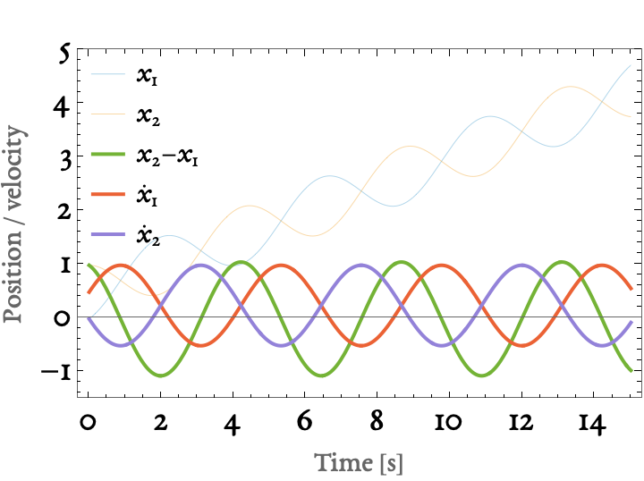
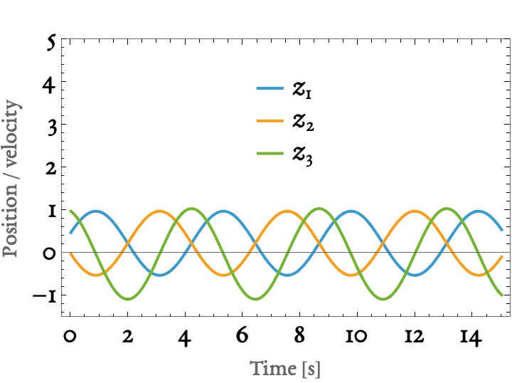
The one on the left was produced using numerical solution of Equation 4, and the one on the right was produced using numerical solution of Equation 5. You can see that \(z_1\) is identical to \(\dot{x}_1\), \(z_2\) is identical to \(\dot{x}_2\), and \(z_3\) is identical to \(x_2-x_1\). While this was not obvious from Figure 1, it has been made obvious in the figure above by plotting three extra quantities: the velocities of the two masses and the difference in their position, both as functions of time. We have basically computed the same information in two different ways.
3.2.1 Code
You can reproduce a version of the figures above using the following code.
% Define the system of ODEs
% y(1) = x1, y(2) = dx1/dt, y(3) = x2, y(4) = dx2/dt
function dydt = odefun(t,y)
    % Parameters
    m1 = 1; m2 = 1; k = 1;

    % Unpack
    x1      = y(1);
    x1dot   = y(2);
    x2      = y(3);
    x2dot   = y(4);

    % Define rhs of diff. eq.
    dydt = [x1dot;
            k*(x2-x1)/m1;
            x2dot;
            -k*(x2-x1)/m2];
end

% Solve
[t, sol] = ode45(@odefun, [0,15], [0; 0.5; 1; 0]);

% Extract results for plotting
x1 = sol(:,1);
v1 = sol(:,2);
x2 = sol(:,3);
v2 = sol(:,4);
diff_x = x2 - x1;

% Create the plot
figure(1); clf;
hold on;

plot(t, x1, 'r-', 'LineWidth', 0.5);      % x1
plot(t, x2, 'b-', 'LineWidth', 0.5);      % x2
plot(t, diff_x, 'k-', 'LineWidth', 2);   % x2 - x1
plot(t, v1, 'r-', 'LineWidth', 2);      % x1_dot
plot(t, v2, 'b-', 'LineWidth', 2);      % x2_dot

% Formatting
xlabel('Time [s]', 'FontSize', 16, 'FontName', 'EB Garamond');
ylabel('Position / velocity', 'FontSize', 16, 'FontName', 'EB Garamond');
grid on; grid minor;
set(gca, 'FontSize', 14, 'FontName', 'EB Garamond');
ylim([-1.5, 5]);

legend({'x_1', 'x_2', 'x_2-x_1', 'dx_1/dt', 'dx_2/dt'}, ...
    'Location', 'northwest', 'FontSize', 12);
% Define the system of ODEs
% y(1) = z1, y(2) = z2, y(3) = z3
function dydt = odefun(t, y)
% Parameters
m1 = 1;
m2 = 1;
k = 1;
% Unpack
z1 = y(1);
z2 = y(2);
z3 = y(3);
% Define rhs of diff. eq.
% z1' = (k/m1) * z3
% z2' = -(k/m2) * z3
% z3' = z2 - z1
dydt = [(k/m1) * z3;
-(k/m2) * z3;
z2 - z1];
end
% Solve
% Initial conditions: z1[0]=0.5, z2[0]=0, z3[0]=1
[t, sol] = ode45(@odefun, [0, 15], [0.5; 0; 1]);
% Extract results for plotting
z1 = sol(:,1);
z2 = sol(:,2);
z3 = sol(:,3);
% Create the plot
figure(1); clf;
hold on;
% Plotting results
plot(t, z1, 'r-', 'LineWidth', 2); % z1
plot(t, z2, 'b-', 'LineWidth', 2); % z2
plot(t, z3, 'k-', 'LineWidth', 2); % z3
% Format
set(gca, 'FontSize', 14);
xlabel('Time [s]');
ylabel('Position / velocity');
grid on; grid minor;
ylim([-1.5, 5]);
legend({'z_1', 'z_2', 'z_3'}, ...
'Location', [0.5, 0.7, 0.1, 0.1]);