Lecture 19
E12 Linear Physical Systems Analysis
Frequency Response
We use the term frequency response to refer to
“the output of a system when the input is a pure sinusoid”
| Order | Input \(f(t)\) | \(F(s)\) | Response \(X(s)\) | Response \(x(t)\) |
|---|---|---|---|---|
1st  |
\(u_s(t) \cdot \sin \omega t\) | \(\displaystyle \frac{\omega}{s^2+\omega^2}\) | \(\displaystyle \frac{\omega}{s^2+\omega^2} \frac{1}{s+a}\) |  |
2nd 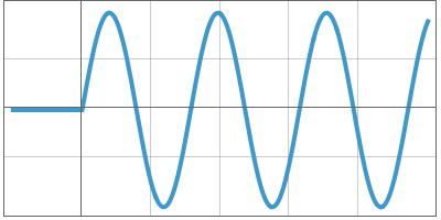 |
\(u_s(t) \cdot \sin \omega t\) | \(\displaystyle \frac{\omega}{s^2+\omega^2}\) | \(\displaystyle \left(\frac{\omega}{s^2+\omega^2} \right) \frac{\omega_n^2}{s^2 + 2 \zeta \omega_n s + \omega_n^2}\) |   |
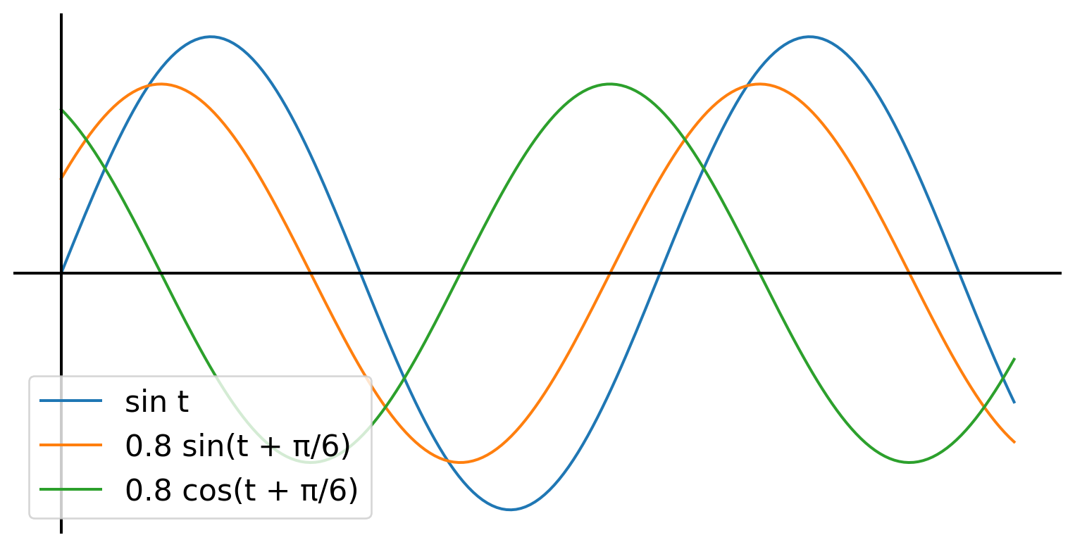
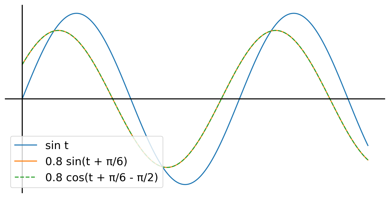
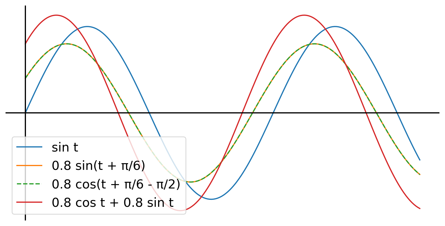
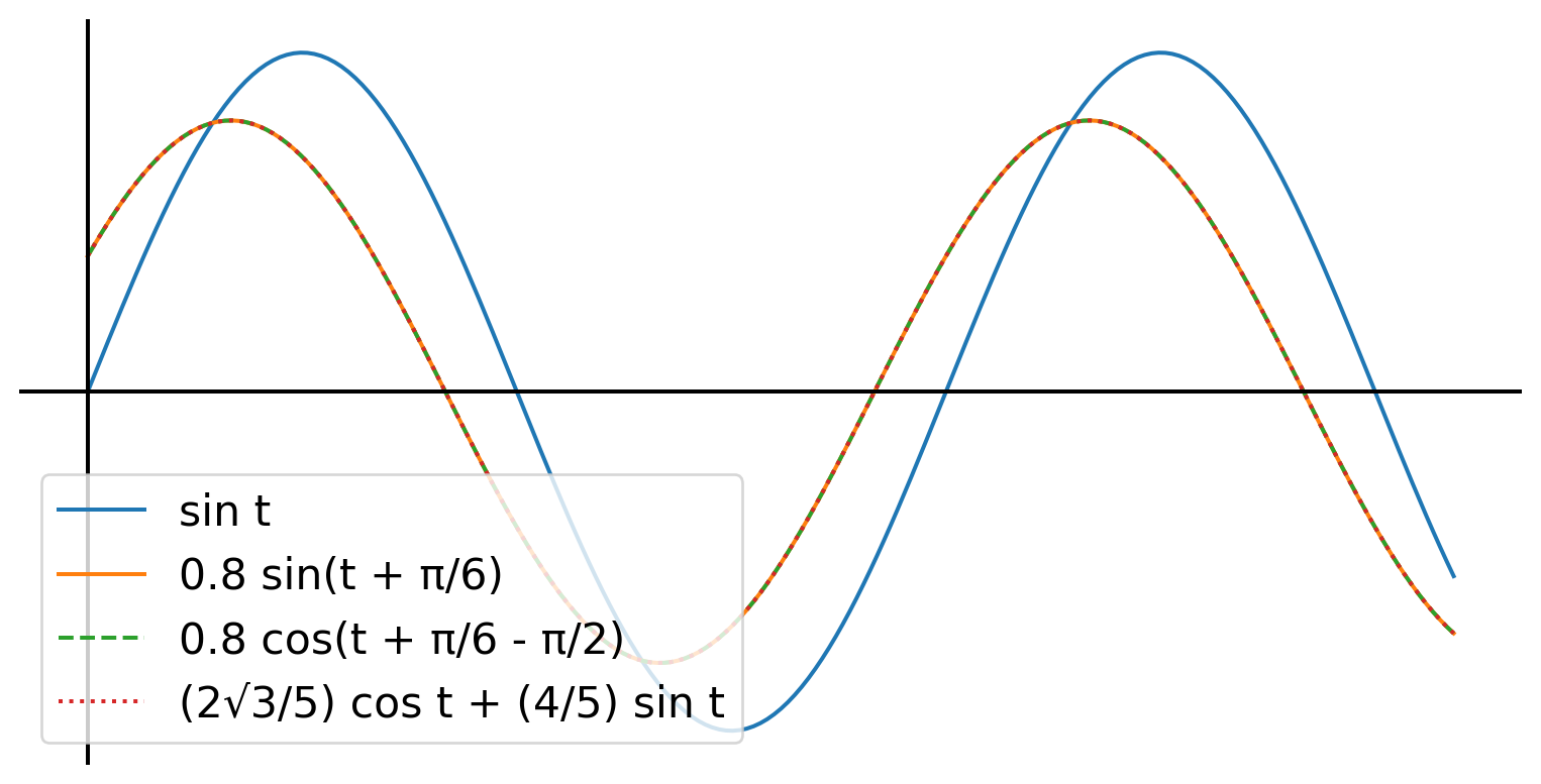
Sines and Shifted Sines
Frequency Response of First Order Systems (in \(s\))
\[\tau \dot{y} + y = f(t)\]
\[\tau s Y(s) + Y(s) = F(s)\]
\[\frac{Y(s)}{F(s)} = \frac{1}{\tau s + 1}\]
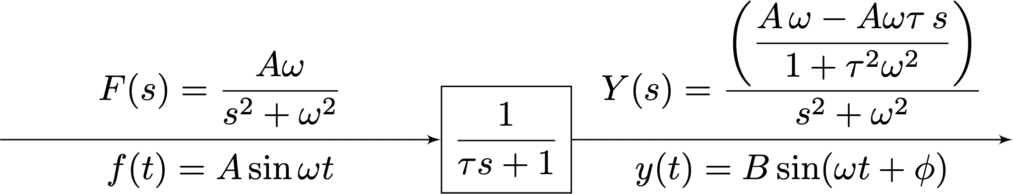
If \(f(t) = A \sin \omega t\),
\[\begin{aligned}F(s) = \frac{A \omega}{s^2 + \omega^2} \implies Y(s) &= \frac{1}{\tau s + 1} \cdot \frac{A \omega}{s^2 + \omega^2} \\ &= \frac{1/\tau}{s + 1/\tau} \cdot \frac{A \omega}{s^2 + \omega^2}\end{aligned}\]
We now have the response of a first order system to a sinusoidal input with frequency \(\omega\) and amplitude \(A\), a.k.a., the frequency response of a first-order system.
Frequency Response of 1st Order Systems (in \(s\))
We would like to take the inverse Laplace Transform
\[\mathcal{L}^{-1} \left[ \frac{1/\tau}{s + 1/\tau} \cdot \frac{A \omega}{s^2 + \omega^2}\right]\]
We use a special trick in partial fractions:
\[\frac{1/\tau}{s + 1/\tau} \cdot \frac{A \omega}{s^2 + \omega^2} = \frac{P}{s+1/\tau} + \frac{Q s + R}{s^2 + \omega^2}\]
And solve for \(P\), \(Q\) and \(R\) by equating coefficients of \(s^0\), \(s^1\) and \(s^2\)
\[ \frac{(1/\tau)(A\omega)}{(s+1/\tau)(s^2+\omega^2)} = \frac{P (s^2+\omega^2) + (Qs+R)(s+1/\tau)}{(s+1/\tau)(s^2+\omega^2)} \]
\[\implies Ps^2 + Q s^2 + Rs + Qs/\tau + R/\tau = 0 s^2 + 0 s + \frac{A \omega}{\tau}\]
after some math….
\[P = \frac{A \tau \omega}{1+\tau^2\omega^2}, \quad Q = \frac{- A \tau \omega}{1+\tau^2\omega^2}, \quad R = \frac{A \omega}{1+\tau^2 \omega^2}\]
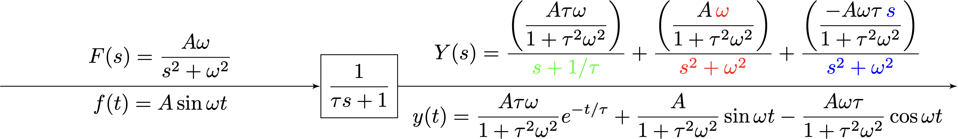
Frequency Response of 1st Order Systems (in \(t\))
We can now write \(Y(s)\) in a form convenient for \(\mathcal{L}^{-1}\):
\[Y(s) = \frac{\left( \displaystyle \frac{ A \tau \omega}{ 1+\tau^2\omega^2}\right)}{\color{green}{s+1/\tau}} + \frac{\left(\displaystyle \frac{A \, \color{red}{\omega}}{1+\tau^2 \omega^2} \right)}{\color{red}{s^2+\omega^2}} + \frac{\left(\displaystyle \frac{ - A \omega \tau \, \color{blue}{s}}{1+\tau^2 \omega^2} \right)}{\color{blue}{s^2+\omega^2}}\]
Recall that the table of Laplace Transform pairs has \[\mathcal{L}^{-1} \left[ \frac{1}{\color{green}{s+a}} \right] = e^{-at}, \quad \mathcal{L}^{-1} \left[ \frac{\color{red}{\omega}}{\color{red}{s^2+\omega^2}} \right] = \sin \omega t, \quad \mathcal{L}^{-1} \left[ \frac{\color{blue}{s}}{\color{blue}{s^2+\omega^2}} \right] = \cos \omega t\]
So the Inverse Laplace Transform gives us an exponential, a sine and a cosine.
Therefore, in the time domain, we have \[y(t) = \frac{A \tau \omega}{1+\tau^2 \omega^2} e^{-\displaystyle \frac{t}{\tau}} + \frac{A}{1+\tau^2 \omega^2 } \sin \omega t - \frac{A \omega \tau}{1+\tau^2 \omega^2} \cos \omega t\]
and we can collect terms to write \[ y(t) = \frac{A \omega \tau}{1+\tau^2 \omega^2} \left[ \overbrace{e^{- t/\tau}}^{\text{transient}} \overbrace{- \cos \omega t + \frac{1}{\omega \tau} \sin \omega t }^{\text{steady state}}\right] \]
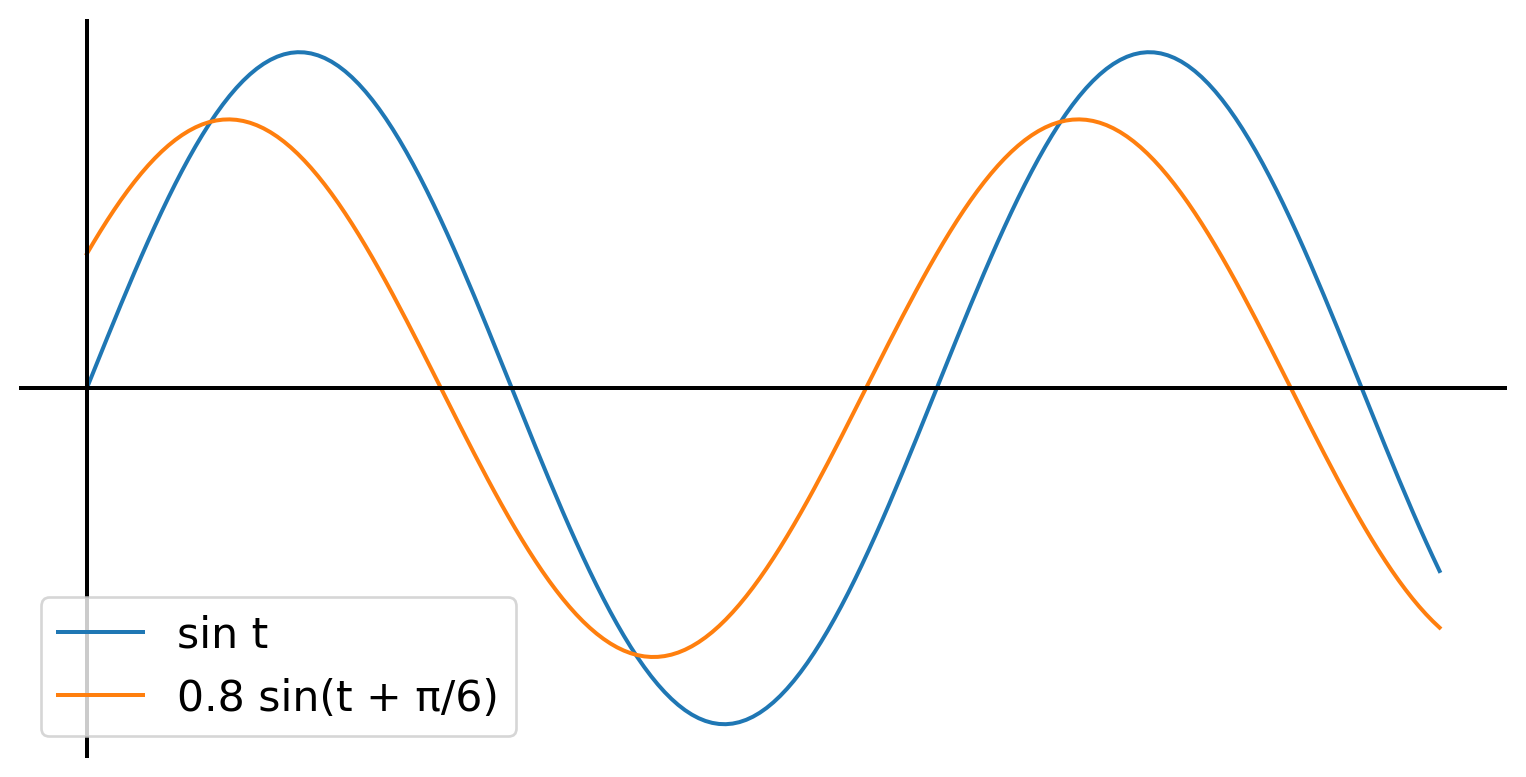
So, we learn that the steady state response of a first-order system to a sinusoidal input is a sine plus a cosine
Steady-State Response of First-order system to sinusoidal input
At long times, \(e^{-t/\tau} \rightarrow 0\)
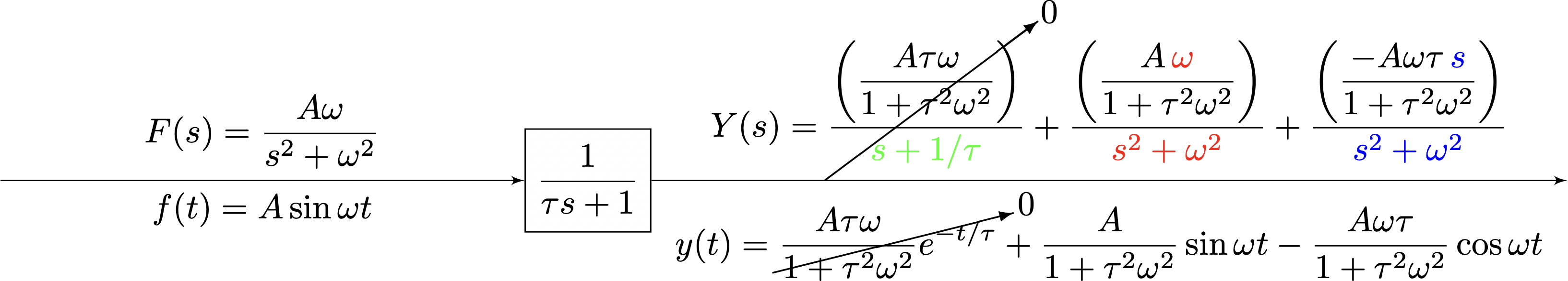
and we can simplify \(y(t) = \frac{A}{1+\tau^2 \omega^2} \left( \sin \omega t - \omega \tau \cos \omega t \right)\) \(= B \sin (\omega t + \phi)\)
because a sine plus a cosine is equal to a phase-shifted sine.
Next, we will learn how to calculate the phase-shift \(\phi\) and amplitude \(B\).
Steady-state frequency response amplitude \(B\)
\[\frac{A}{1+\tau^2 \omega^2} \left( \sin \omega t - \omega \tau \cos \omega t \right) = {\color{brown}{\frac{A}{1+\tau^2 \omega^2}}}\sin \omega t {\color{magenta}{- \frac{A \omega \tau }{1+\tau^2 \omega^2}}} \cos \omega t = B \sin (\omega t + \phi)\]
A trigonometric identity tells us that \[B \sin (\omega t + \phi) = {\color{brown}{B \cos \phi }}\sin \omega t + {\color{magenta}{B \sin \phi }} \cos \omega t\]
and we can equate the brown and magenta terms respectively: \[{\color{brown}{B \cos \phi = \frac{A}{1+\tau^2 \omega^2}}}, \quad {\color{magenta}{B \sin \phi = -\frac{A \omega \tau}{1+\tau^2 \omega^2}}}\]
Square them and sum them \[B^2 \left( \cos^2 \phi + \sin^2 \phi \right) = \left( \frac{A}{1+\tau^2 \omega^2} \right)^2 + \left( -\frac{A \omega \tau}{1+\tau^2 \omega^2}\right)^2\]
\[= \frac{A^2 + A^2 \omega^2 \tau^2}{\left( 1+\omega^2 \tau^2 \right)^2} = \frac{A^2\left( 1 + \omega^2 \tau^2 \right) }{\left( 1+\omega^2 \tau^2 \right)^2} \]
\[\implies B^2 = \frac{A^2}{1+\omega^2 \tau^2}\]
So the amplitude of the steady-state output is \[\displaystyle B = \boxed{\frac{A}{\sqrt{1+\omega^2 \tau^2}}}\]
Formula for steady-state frequency response phase shift \(\phi\)
\[B \sin \phi = \frac{-A \omega \tau}{1+\omega^2 \tau^2}\] \[B \cos \phi = \frac{A}{1+\omega^2 \tau^2}\]
\[ \begin{aligned} \tan \phi &= \left(\frac{-A \omega \tau}{1+\omega^2 \tau^2}\right) \div \left(\frac{A}{1+\omega^2 \tau^2}\right) \\ \tan \phi &= (- \omega \tau) \\ \implies \phi &= \boxed{\tan^{-1} (-\omega \tau)} \end{aligned} \]
An example
A first-order system \(\tau \dot{y} + y = f(t)\) with time constant \(\tau = 5\) seconds is given an input of \(f(t) = \sin 3t\).
In-class questions:
- What kind of function is the steady-state response?
- Answer: Shifted sine
- Write down the steady-state response as a function of time.
- Answer: \(y(t) = B \sin (\omega t + \phi)\)
\[ \begin{aligned} B &= \frac{A}{\sqrt{1+\omega^2 \tau^2}} \\ \phi &= \tan^{-1} (-\omega \tau) \end{aligned} \]
\[ \begin{aligned} B &= \frac{A}{\sqrt{1+\omega^2 \tau^2}} \\ &= \frac{1}{\sqrt{1+3^2 \times 5^2}} \\ &= \frac{1}{\sqrt{1+225}} = \frac{1}{\sqrt{226}} \approx 0.06652 \end{aligned} \]
\[ \begin{aligned} \phi &= \tan^{-1} (-\omega \tau) \\ &= \tan^{-1}(-3 \cdot 5) & \approx -1.504 \end{aligned} \]
\[ \boxed{\overbrace{\sin 3 t}^{\text{input}} \longrightarrow \boxed{\text{system}} \longrightarrow \text{ transient dies} \longrightarrow \overbrace{0.06652 \sin (3t - 1.504)}^{\text{steady-state output}}} \]
Amplitude Ratio & Phase
If the input to a first-order system is \(f(t) = \boxed{A \sin \omega t}\), the steady-state output is \(\boxed{B \sin \omega(t+ \phi)}\)
\[\tau \dot{y} + y = f(t)\]
- Some questions that we might ask:
- What is the amplitude ratio \(B/A\)?
- How much is the phase shift ?
- These quantities depend on two numbers:
- The time constant of the system \(\tau\)
- The frequency of the input applied to it \(\omega\)
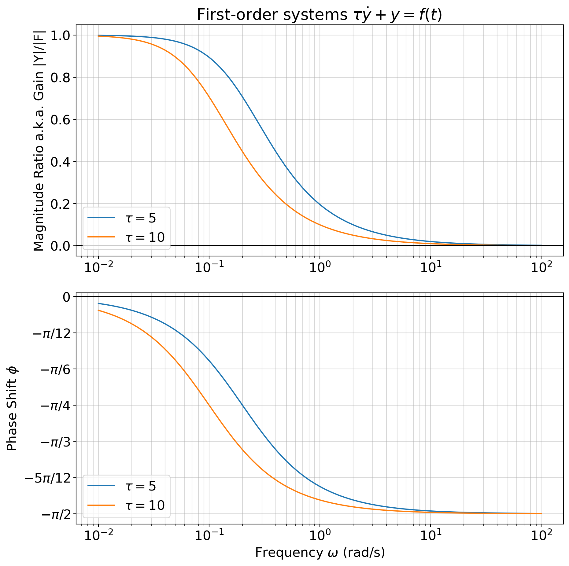
- Amplitude ratio \[M = \frac{|Y|}{|F|} = \frac{1}{\sqrt{1+\omega^2 \tau^2}}\]
- Phase shift \[\phi = \tan^{-1} (- \omega \tau)\]
Using the Transfer Function to determine (s.s.) Frequency Response
The system \[\tau \dot{y} + y = f(t)\] has the transfer function \(T(s)\) given by \[\frac{Y(s)}{F(s)} = T(s) = \frac{1}{\tau s + 1}\]
A pure sinusoidal function corresponds to \(s = 0 + i \omega\)
Substituting \(s=i \omega\) into the transfer function of a system gives us information about the response of that system to a sinusoidal input.
\[T(i \omega) = \frac{1}{i \omega \tau + 1}\]
- Note: \(T(i\omega)\) is a complex number for any given \(\omega\)
- The amplitude ratio (a.k.a. gain) is given by the magnitude of this complex number \(|T(i\omega)|\)
- The phase shift is given by the argument of this complex number \(\arg T(i\omega)\)
Bode Plots of First-order Systems