Lecture 24
E12 Linear Physical Systems Analysis
Plan for week 14 (fill out poll on EdStem!)
Comprehensive Final Assigment in class on Thursday to synthesize everything we have learned
No HW will be assigned on week 14
Tuesday:
- Instructor analyzes an electrical system on board
Thursday:
- You will analyze a mechanical system in class and turn in your work, including some/all of:
- State variables
- Differential Equation
- Laplace Transform
- Block Diagram
- Transfer Function
- Free Response
- Step Response
- Impulse Response
- Frequency Response
- Bode Plots
Developing state-space equations

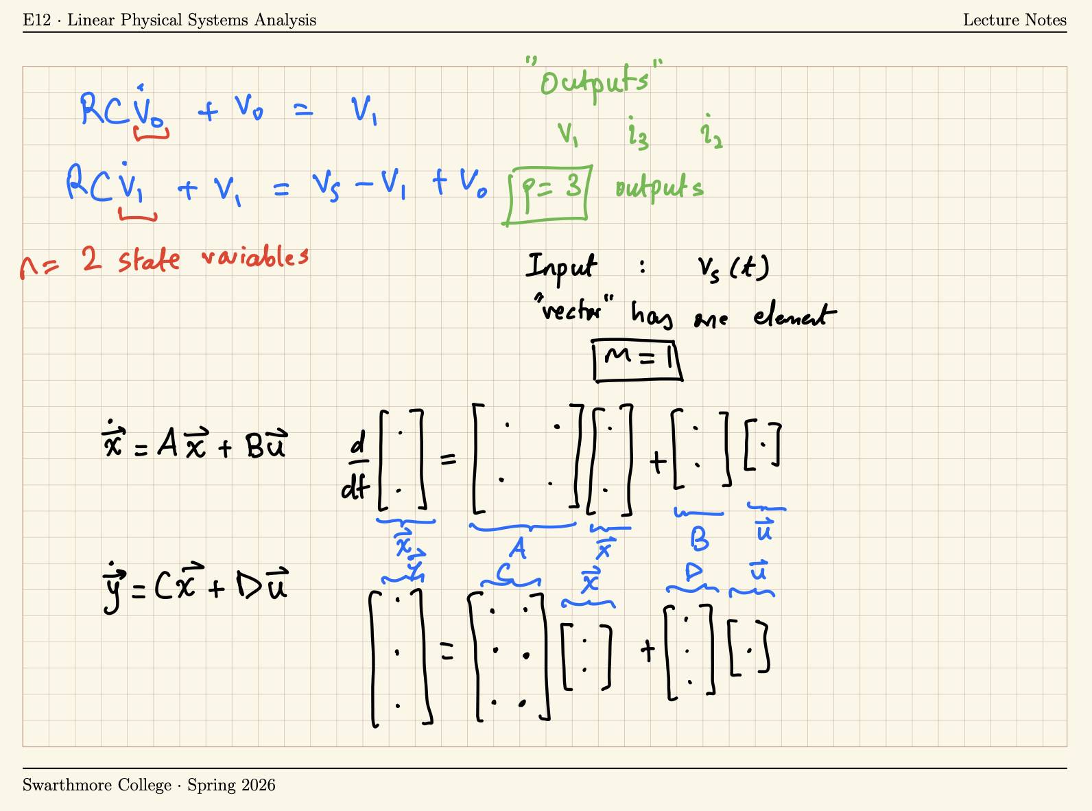
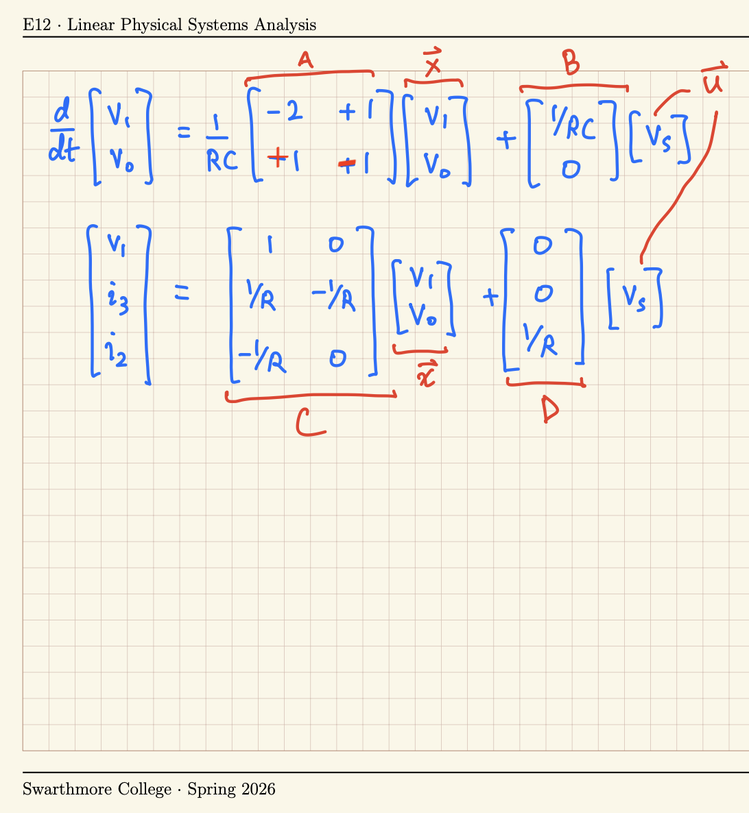
We are interested in the outputs: \(v_1\), \(i_3\) and \(i_2\).
A circuit with three outputs and one input
State-Space Models in MATLAB
We use the term ‘state space equations’ to refer to the set
\[\dot{\boldsymbol{x}} = \boldsymbol{A} \boldsymbol{x} + \boldsymbol{B} \boldsymbol{u} \tag{1}\]
\[{\boldsymbol{y}} = \boldsymbol{C} \boldsymbol{x} + \boldsymbol{D} \boldsymbol{u} \tag{2}\]
MATLAB has a built-in function that allows us to construct a sytem in state space form
where the matrices A, B, C and D are as defined in Equation 3 and Equation 4.
Functions Available in MATLAB for state-space models
Given a ‘state-space object’ created using system1 = ss(A,B,C,D)
tf(system1)– obtain the transfer functions for this systemstep(system1)– graph the step responseimpulse(system1)– graph the impulse responselsim(system1,u,t)– graph the response to an arbitrary input \(u(t)\) given as vectorsuandtbodeplot(system1– generate a Bode plot in deciBels (see Lab 5)
Multiple inputs, Multiple outputs
\[\dot{\boldsymbol{x}} = \boldsymbol{A} \boldsymbol{x} + \boldsymbol{B} \boldsymbol{u} \tag{3}\]
\[{\boldsymbol{y}} = \boldsymbol{C} \boldsymbol{x} + \boldsymbol{D} \boldsymbol{u} \tag{4}\]
If there are two inputs and two outputs, determine the size/shape of A, B, C and D. Also determine how many transfer functions are needed to describe this system. Assume there are four state variables in this system.
\[ A = \begin{bmatrix} 0 & 1 & 0 & 0 \\ -1 & -12/5 & 4/5 & 8/5 \\ 0 & 0 & 0 & 1 \\ 4/3 & 8/3 & -4/3 & -8/3 \end{bmatrix}, \quad B = \begin{bmatrix} 0 & 1 \\ 0 & 0 \\ 0 & 0 \\ 1/3 & 0 \end{bmatrix} \]
\[ C = \begin{bmatrix} 1 & 0 & 0 & 0 \\ 0 & 0 & 1 & 0 \end{bmatrix}, \quad D = \begin{bmatrix} 0 & 0 \\ 0 & 0 \end{bmatrix} \]
Example
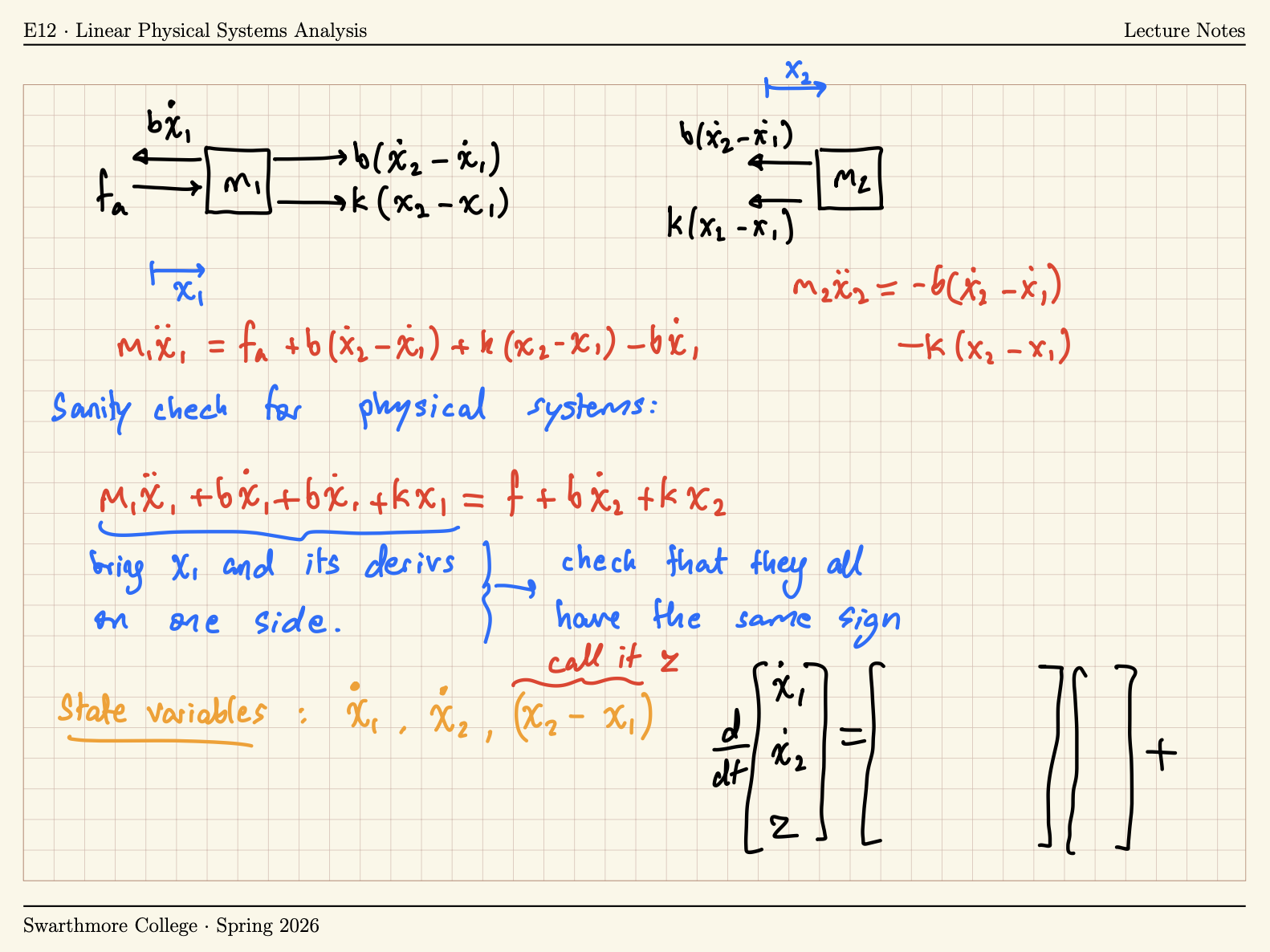
Use the state-space model to determine the effect on the quantity \((x_2-x_1)\) of pushing \(m_1\) with suddenly to the right, when
- \(m=1\), \(k=3\), and \(b = 5\)
- \(m=1\), \(k=3\), and \(b=0.2\)

Procedure:
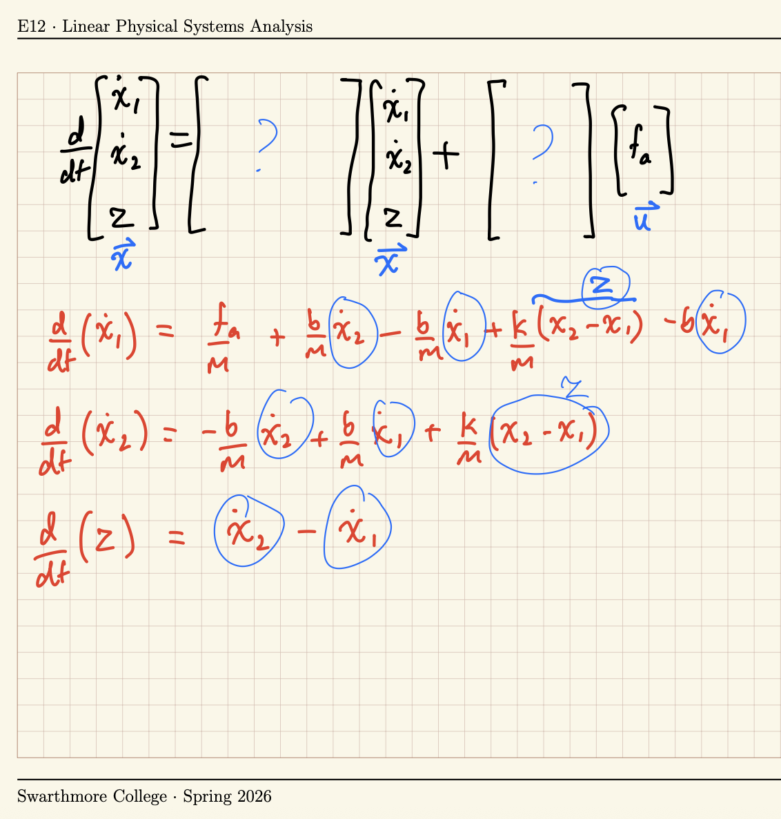
- Determine state variables
- Write the state-variable equation \(\dot{\boldsymbol{x}} = \boldsymbol{A} \boldsymbol{x} + \boldsymbol{B} \boldsymbol{u}\)
- Write the output equation \({\boldsymbol{y}} = \boldsymbol{C} \boldsymbol{x} + \boldsymbol{D} \boldsymbol{u}\)
- Gather matrices A, B, C and D and use
ssto make state-space model - Use
impulsefunction.
Example