Lecture 24
E12 Linear Physical Systems Analysis
April 16, 2026
Plan for week 14 (fill out poll on EdStem!)
- State variables
- Differential Equation
- Laplace Transform
- Block Diagram
- Transfer Function
- Free Response
- Step Response
- Impulse Response
- Frequency Response
- Bode Plots
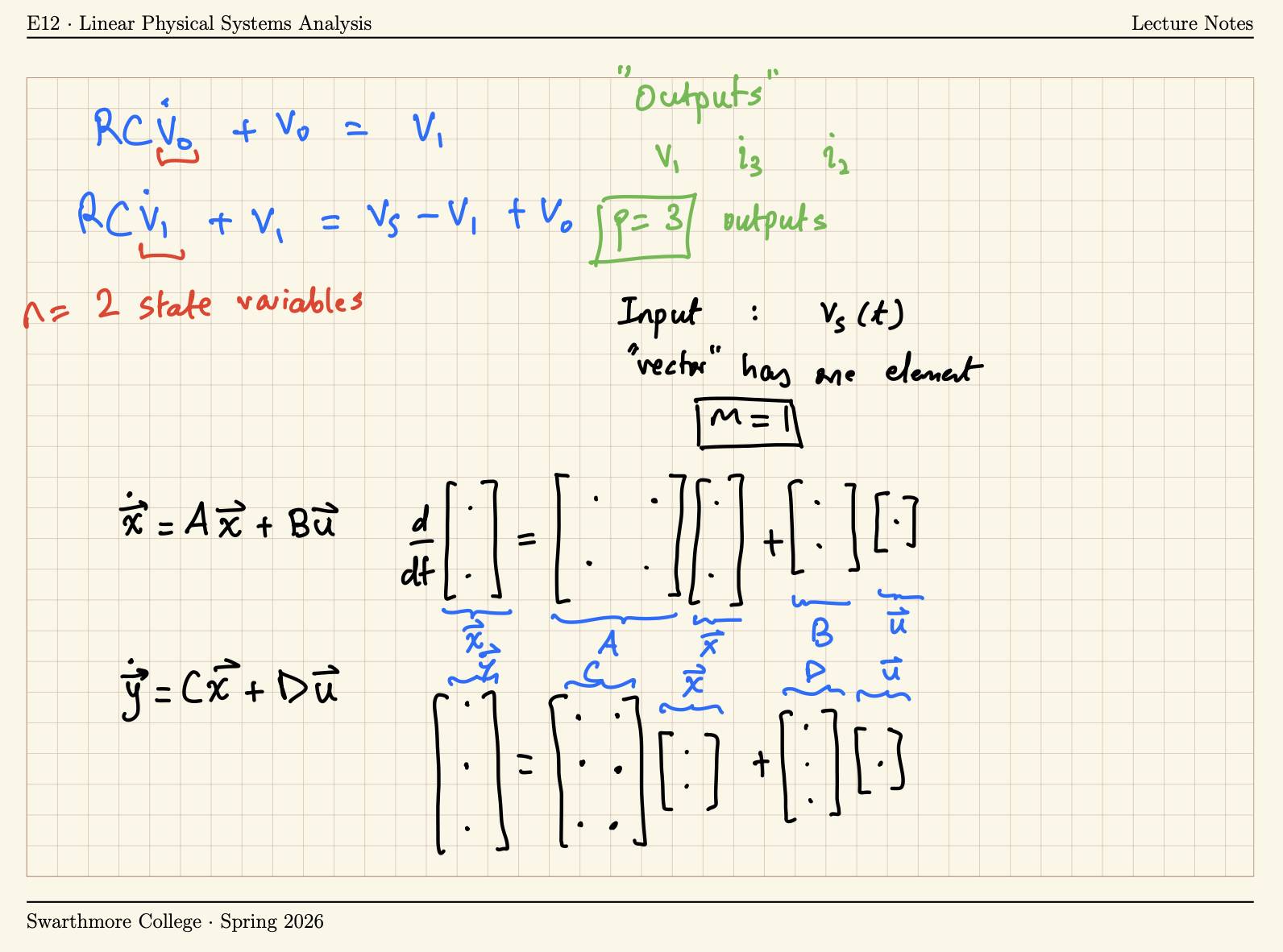
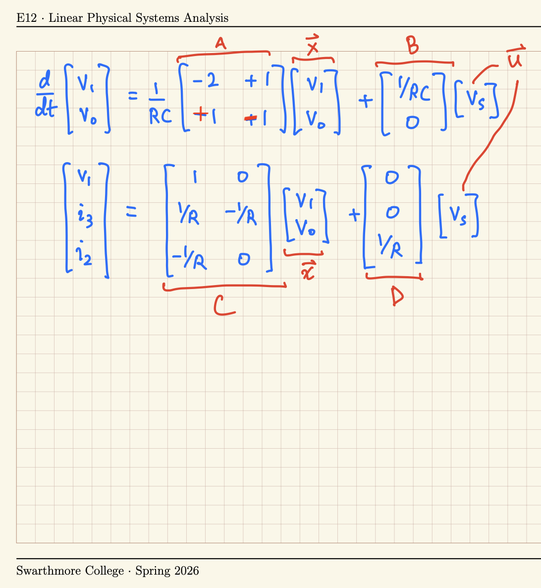
Developing state-space equations
![]()
We are interested in the outputs: \(v_1\), \(i_3\) and \(i_2\).
State-Space Models in MATLAB
We use the term ‘state space equations’ to refer to the set
\[\dot{\boldsymbol{x}} = \boldsymbol{A} \boldsymbol{x} + \boldsymbol{B} \boldsymbol{u} \tag{1}\]
\[{\boldsymbol{y}} = \boldsymbol{C} \boldsymbol{x} + \boldsymbol{D} \boldsymbol{u} \tag{2}\]
MATLAB has a built-in function that allows us to construct a sytem in state space form
Functions Available in MATLAB for state-space models
Given a ‘state-space object’ created using system1 = ss(A,B,C,D)
tf(system1) – obtain the transfer functions for this systemstep(system1) – graph the step responseimpulse(system1) – graph the impulse responselsim(system1,u,t) – graph the response to an arbitrary input \(u(t)\) given as vectors u and tbodeplot(system1 – generate a Bode plot in deciBels (see Lab 5)
Example
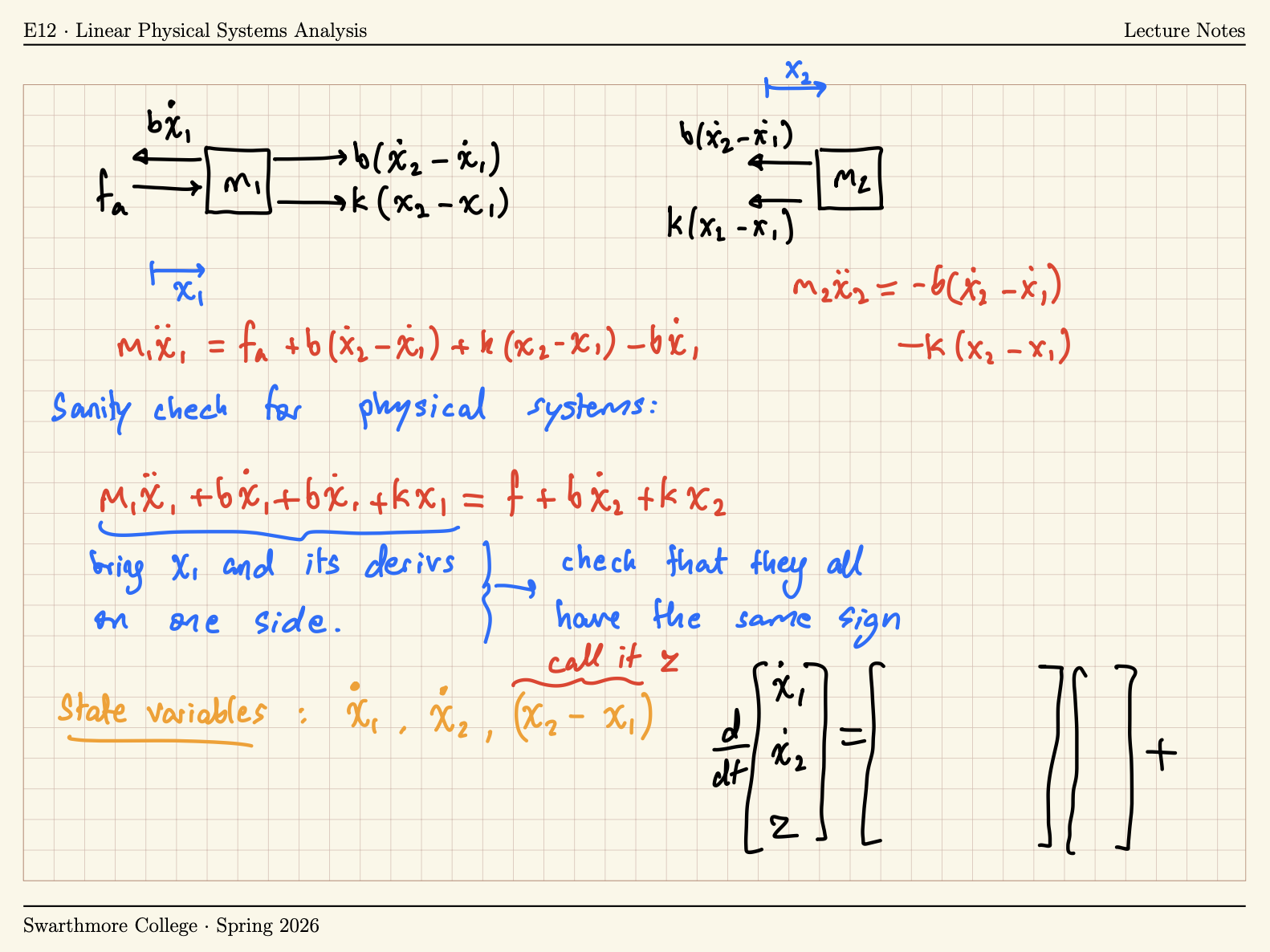
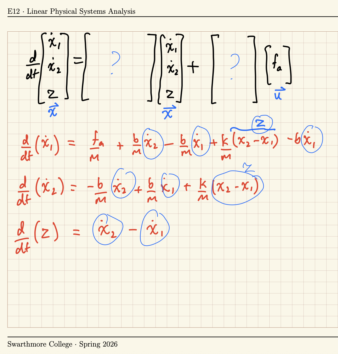
Use the state-space model to determine the effect on the quantity \((x_2-x_1)\) of pushing \(m_1\) with suddenly to the right, when
- \(m=1\), \(k=3\), and \(b = 5\)
- \(m=1\), \(k=3\), and \(b=0.2\)
Procedure:
- Determine state variables
- Write the state-variable equation \(\dot{\boldsymbol{x}} = \boldsymbol{A} \boldsymbol{x} + \boldsymbol{B} \boldsymbol{u}\)
- Write the output equation \({\boldsymbol{y}} = \boldsymbol{C} \boldsymbol{x} + \boldsymbol{D} \boldsymbol{u}\)
- Gather matrices A, B, C and D and use
ss to make state-space model
- Use
impulse function.