Lecture 10
E12 Linear Physical Systems Analysis
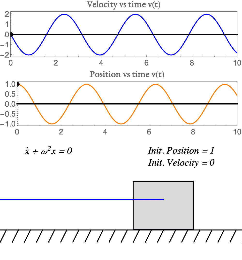
The Natural Frequency
Second-order systems have a natural tendency to oscillate. The frequency at which this occurs is called the natural frequency.
| Symbol | Quantity | Units | Definition |
|---|---|---|---|
| \(\omega\) or \(\omega_n\) | Natural (angular) frequency | \(\mathrm{rad} s^{-1}\) | \(\omega = \sqrt{k/m}\) |
| \(f\) or \(f_n\) | Natural frequency | \(s^{-1}\) | \(\omega = 2 \pi f\) |
| \(T\) | Period | \(s\) | \(2\pi/\omega\) |
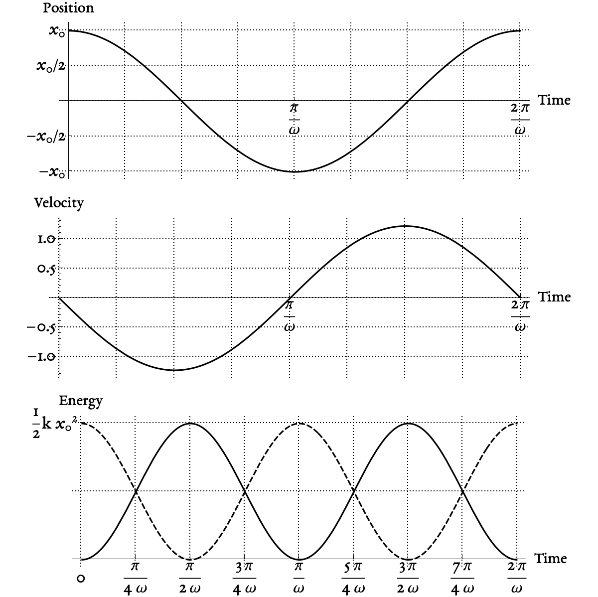
Energy Considerations in the Free Response
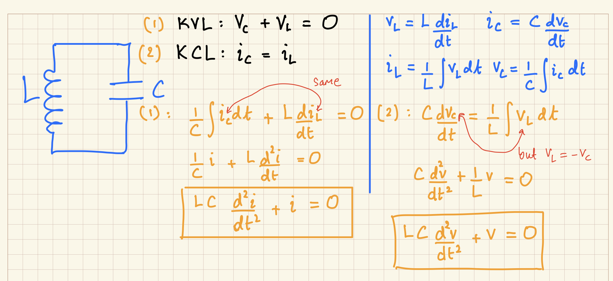
Where else do second-order systems arise?
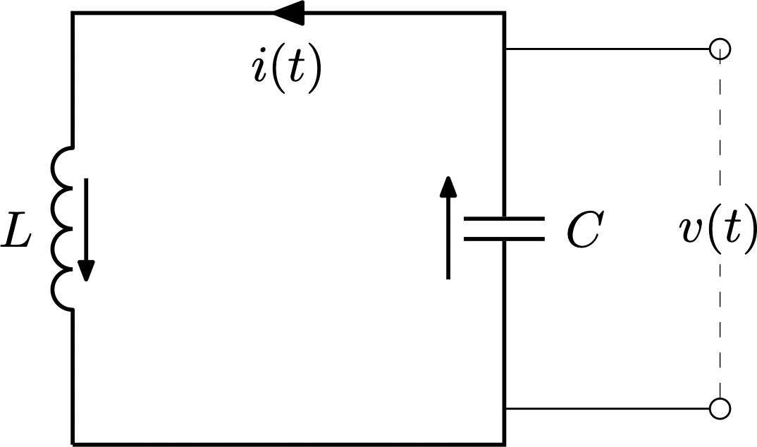
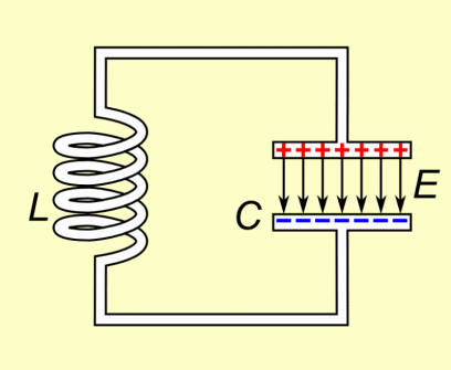
- Applying Kirchhoff’s Laws:
\(\displaystyle \boxed{LC\frac{d^2 i}{dt^2} + i = 0}\)
\(\displaystyle \boxed{LC\frac{d^2 v}{dt^2} + v = 0}\)
Derivation of equations for LC Circuits
Second-order systems in the frequency domain
\[\ddot{x} + \omega^2 x = f(t) \tag{1}\]
Taking the Laplace Transform, we get \[s^2 X + \omega^2 X = F\]
We can therefore write the transfer function as \[\frac{X(s)}{F(s)} = \frac{1}{s^2 + \omega^2}\]
Recall: The transfer function of a system is also its ‘impulse response’
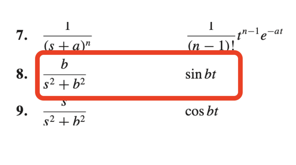
Impulse Response of system in Equation 1 is: \[\frac{1}{s^2+\omega^2} = \frac{1}{\omega} \frac{\omega}{s^2+\omega^2}\]
The Impulse Response of \(\ddot{x}+\omega^2 x = f(t)\) is a sine function
\[\frac{X(s)}{F(s)} = \frac{1}{s^2+\omega^2} = \frac{1}{\omega} \frac{\omega}{s^2+\omega^2}\]

What is the amplitude and period?
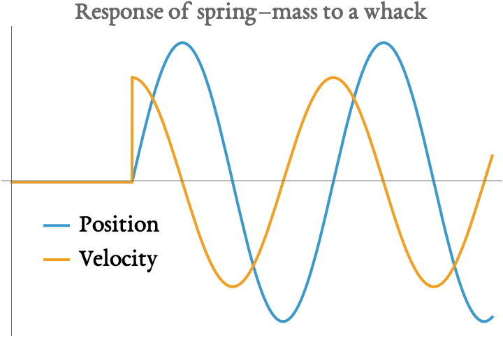
The impulse response of a 2nd order system
\[m \ddot{x} + k x = f(t)\] \[f(t) = \delta(t)\]

In-class task: Find the impulse response in (1) the time domain and (2) the frequency domain.
Impulse response: “An expression in terms of (1) \(t\) and (2) \(s\) that describes how this system behaves when \(f(t) = \delta(t)\), the unit impulse.”
Recall: The unit impulse response is the transfer function
Answer: \[ \frac{X(s)}{F(s)} = \frac{1}{ms^2 + k} = \frac{1/m}{s^2 + k/m} = \frac{1}{\sqrt{mk}} \frac{\omega}{s^2+\omega^2} \]
In the time domain: \(\displaystyle \quad \frac{1}{\sqrt{mk}} \sin \omega t\)
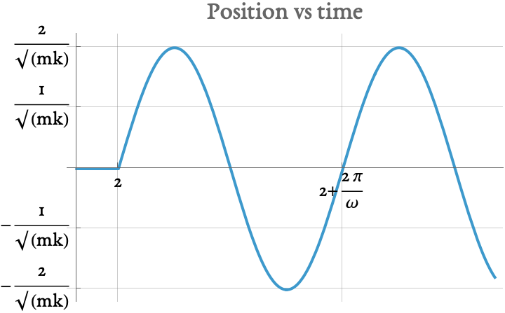
Putting some numbers on it
\[m \ddot{x} + k x = f(t)\] \[f(t) \approx 2 \delta(t-t_1)\]
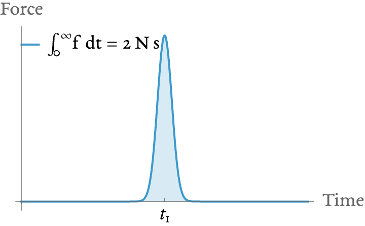
\(m =3.5\mathrm{kg}, k = 1.2 \mathrm{N/m}, t_1 = 2 \mathrm{s}\)
The mass is struck with a force described by the graph above.
In-class task: Sketch a graph of position vs. time (with numbers!)
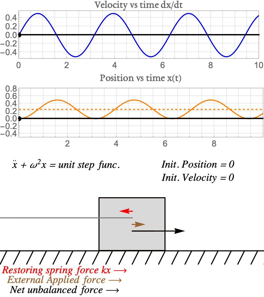
Free and Forced Response
\[\ddot{x} + \omega^2 x = f(t)\]
- Applying the Laplace Transform with \(x(0) \neq 0, \dot{x}(0) \neq 0\) \[ s^2 X - s x(0) - \dot{x}(0) + \omega^2 X = F(s) \\ \implies (s^2+\omega^2)X = F + \dot{x}(0) + s x(0) \]
- Dividing through by \(s^2 + \omega^2\), \[X(s) = \underbrace{\underbrace{\frac{1}{s^2 + \omega^2}}_{\text{T.F.}} F}_{\text{Forced Response}} + \underbrace{\frac{\dot{x}(0)}{s^2 + \omega^2} + \frac{s x(0)}{s^2 + \omega^2}}_{\text{Free Response}}\]
In-class task: Express the Transfer Function as a sum of fractions.
Step Response of a Second-order system
\[ \ddot{x} + \omega^2 x = \begin{cases} a & t > 0 \\ 0 & t < 0 \end{cases} \] \(x(0) = \dot{x} = 0\)
In-class task: If \(a\) is some positive number constant in time, describe the motion of this object.
Step Response of \(\ddot{x} + \omega^2 x = f(t)\)
Calculating the step response of \(\ddot{x} + \omega^2 x = a u_s(t)\)
Step function with magnitude \(a\) applied to r.h.s.
\(\ddot{x} + \omega^2 x = a\)
Procedure in time domain
- Guess a solution: \(x(t) = ba\)
- Substitute: \(\frac{d^2(ba)}{dt^2} + \omega^2 ba = a\)
- \(\implies b = 1/\omega^2\)
- \(x(t) = \frac{a}{\omega^2}\) is a solution to \(\ddot{x} + \omega^2 x = a u_s(t)\)
- Add the solution to \((\ddot{x} + \omega^2 x =0)\) to above
- \(x(t) = \left( x_0 - \frac{a}{\omega^2} \right) \cos \omega t + \frac{v_0}{\omega} \sin \omega t + \frac{a}{\omega^2}\)
\(s^2 X(s) + \omega^2 X(s) = F(s)\)
Procedure in frequency domain
- Take Laplace Transform of \(u_s(t)\)
- Determine forced response as a function of \(s\)
- Use partial fractions
- Convert into time domain using Inverse Laplace Transform.
Spring-Mass system in Simulink
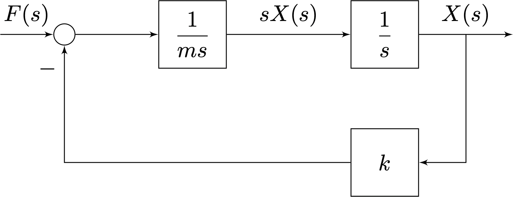
\[ \begin{aligned} m \ddot{x} + kx &= f(t) \\ ms^2 X + k X &= F \\ ms^2 X &= F - k X \\ sX &= \frac{1}{ms} \left( F - k X\right) \\ X &= \frac{1}{s} \underbrace{\left[ \frac{1}{ms} \left( F - k X \right) \right]}_{s X(s) \rightarrow \mathcal{L}^{-1} \rightarrow \dot{x}} \end{aligned} \]
Download model from Website > Resources > Simulink
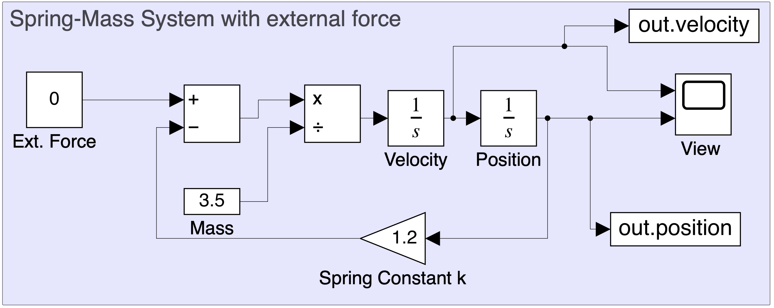
- Block Diagrams help you make Simulink models
- Triangular “Gain” replaces rectangular multiplicative block
- Arithmetic operations made explicit
Using Simulink for 2nd order systems
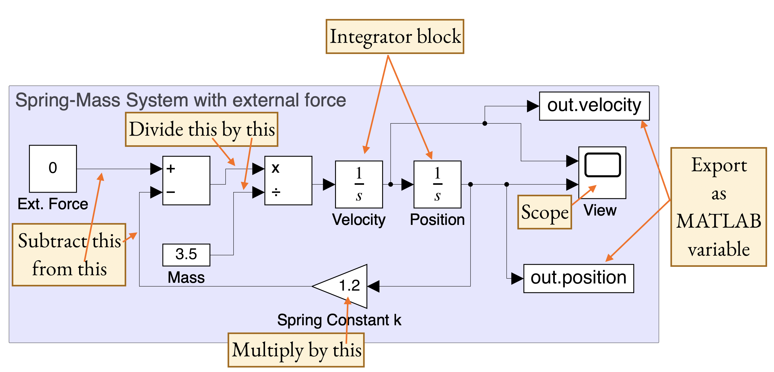
- Check initial conditions by double-clicking integrator blocks
- Specify time step in Simulation Toolbar > Prepare > Model Settings > Solver > Solver Details
- Access output variables in MATLAB using
out.toutfor time,out.velocityandout.position
In-class task: (1) Add a nonzero external force of 5 N. (2) Use Signal Generator block to add a sinusoidal input force.