Problem Set 8 Solutions
ENGR 12, Spring 2026.
Solutions
1 Deriving the equations
Draw correct free-body diagrams and find the governing differential equation(s) for the following system. There should be three second-order differential equations for \(x_1\), \(x_2\) and \(x_3\). Assume that all three lengths are defined such that, when \(x_1=x_2=x_3=0\), there is no restoring force in any of the springs.
Don’t forget the gravity term!
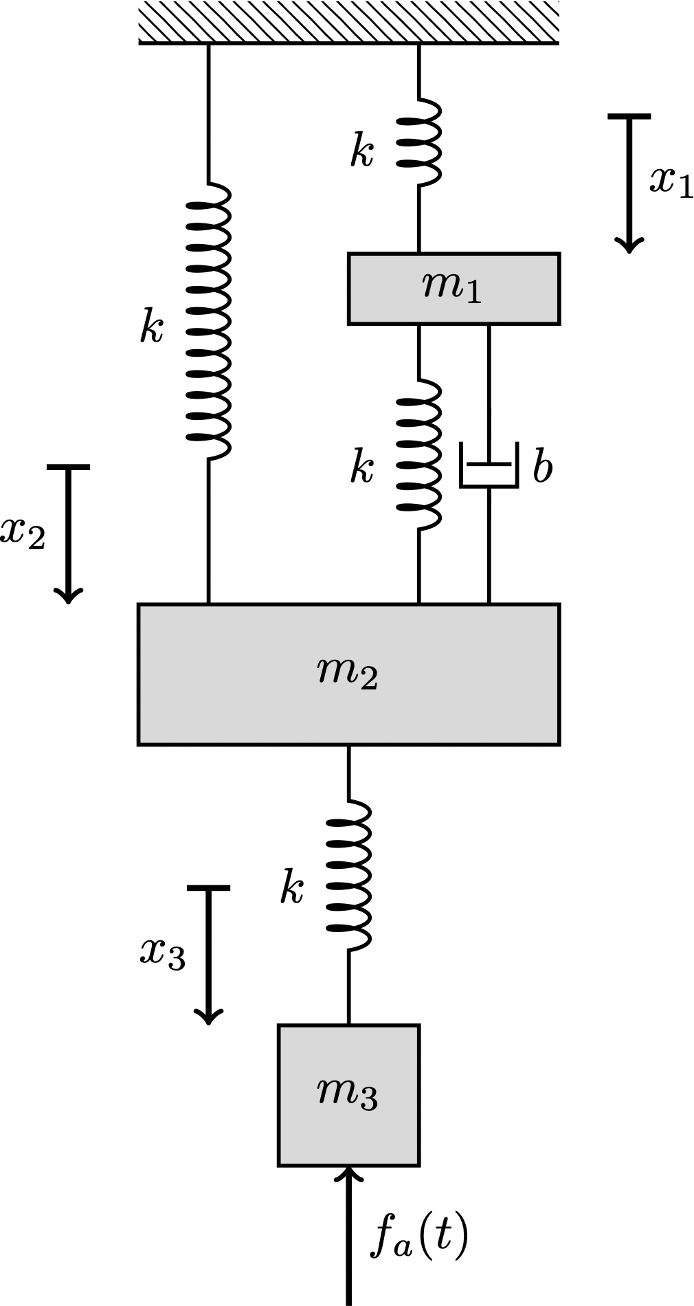
Let us present below the free-body diagrams for each mass. For neatness, we will omit the term \(mg\) from our diagrams, but we will remember to include it in the equations.
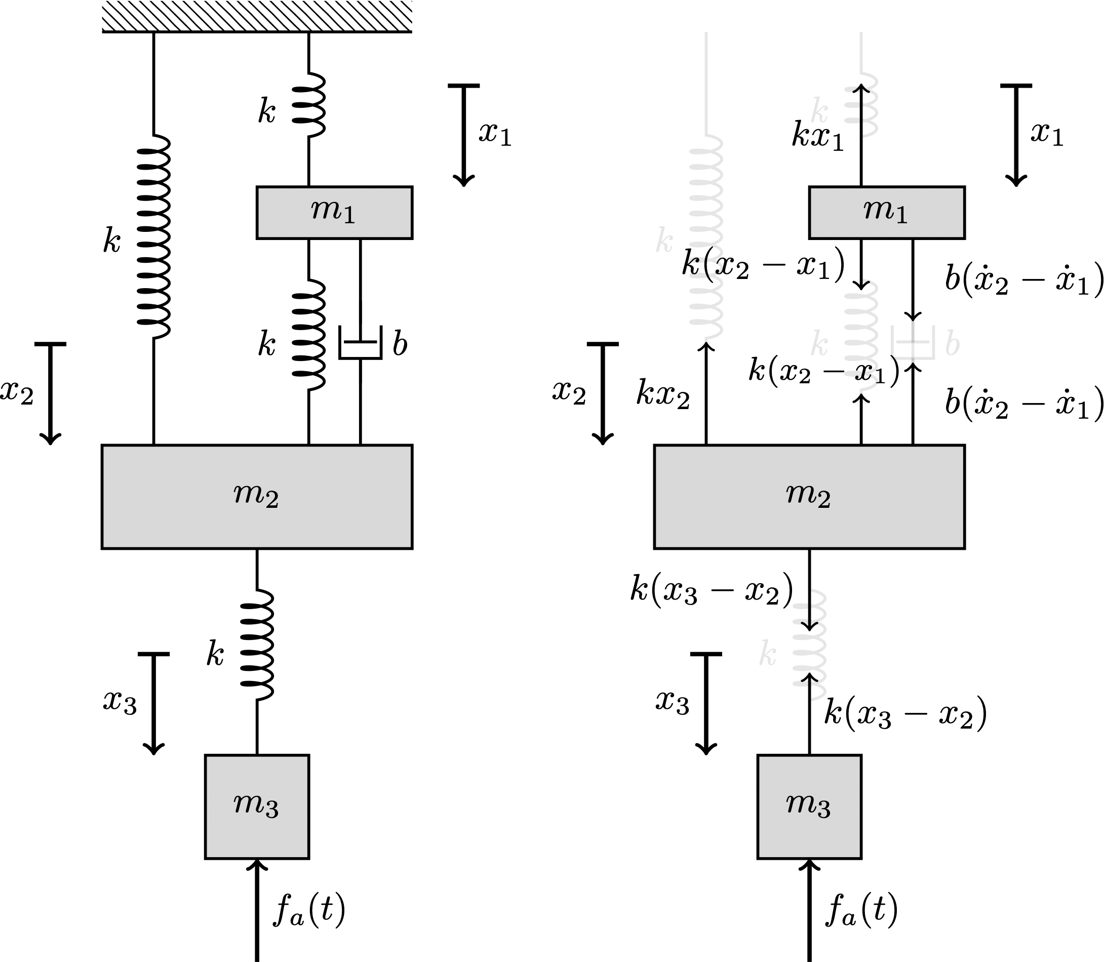
FBD of mass 1: \[m_1 \ddot{x}_1 = k(x_2-x_1) + b (\dot{x}_2-\dot{x}_1) - k x_1 + m_1 g\]
FBD of mass 2: \[m_2 \ddot{x}_2 = k (x_3-x_2) - k x_2 - k (x_2-x_1) - b (\dot{x}_2-\dot{x}_1) + m_2 g\]
FBD of mass 3: \[m_3 \ddot{x} = - f_a(t) + m_3 g - k(x_3-x_2)\]
2 Two Masses on a moving cart
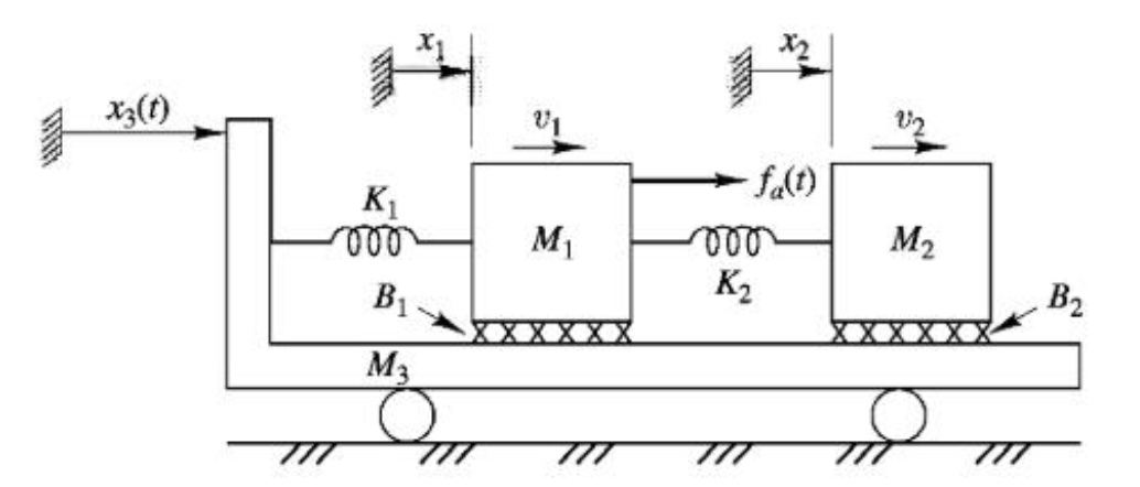
Consider the system shown below, in which two masses \(M_1\) and \(M_2\) are placed on a moving cart with mass \(M_3\). There is friction between the masses and the cart, following the usual ‘element law’ of friction being proportional to the relative velocity between the two surfaces. A force is applied to mass \(M_1\) to the right with magnitude \(f_a(t)\).
2.1 State Variables
Determine the number of state variables in this system and write down mathematical symbols for each of them.
There are five energy-storing elements in this system: the three masses and the two springs. Thus, there appear to be five state variables. They are \(x_1\), \(x_2\), \(\dot{x}_3\), \(\dot{x}_1\) and \(\dot{x}_2\).
2.2 Input Force
For this part, assume that the cart is forced to be at rest at all times and \(x_3(t) = \dot{x}_3(t) = \ddot{x}_3(t) = 0\). The system is put into motion through a force \(f_a(t)\). Ignore initial conditions.
- Draw all relevant free-body diagrams for this system. Your diagrams should have the correct arrows, labels, and signs.
- Write down the governing differential equations for this system.
- Using the state variables that you identified in Section 2.1 or a subset of them, write down the governing differential equations for this system in the form \(\dot{x} = A \ x + b\), where \(x\) is a vector of state variables, \(A\) is the system matrix, and \(b\) contains information about the applied force.
- Use MATLAB to solve this system of equations numerically for an applied force \(f_a(t)\) that is given by the ‘top-hat function’ from HW 7. Generate a plot of the resulting solution and turn in a copy of the modified file
prob12_rhs.m(in the form of a screenshot or text, not a.mfile) as well as an image of the plot. Note that the system should start from rest. You may make use of the skeleton code provided below. The only significant change that you need to make is in the file namedprob12_rhs.m. The parameter values are:
- \(m_1=m_2 = 1\)
- \(k_1=k_2=2\)
- \(b_1=b_2=0.5\)
- Repeat the MATLAB solution with a different value for \(k_1 = 10\), keeping all other parameters the same. Turn in the resulting plot.
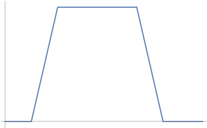
The input as a function of time looks like the following figure:
- TBD
- The governing differential equations are (note that \(x_3 =0\)) \[ \begin{aligned} M_1 \ddot{x}_1 &= f_a(t) + K_2 (x_2-x_1) - K_1 x_1 - B_1 \dot{x}_1 \\ M_2 \ddot{x}_2 &= \phantom{f_a(t) }- K_2 (x_2-x_1) \phantom{-K_1 x_1 } - B_2 \dot{x}_2 \end{aligned} \]
- Using four state variables \(x_1\), \(\dot{x}_1\), \(x_2\) and \(\dot{x}_2\), we can write these equations as \[ \frac{d}{dt} \begin{bmatrix} x_1 \\ \dot{x}_1 \\ x_2 \\ \dot{x}_2 \end{bmatrix} = \begin{bmatrix} 0 & 1 & 0 & 0 \\ \displaystyle -\frac{(K_1 + K_2)}{M_1} & \displaystyle -\frac{B_1}{M_1} & \displaystyle \frac{K_2}{M_1} & 0 \\ 0 & 0 & 0 & 1 \\ \displaystyle \frac{K_2}{M_2} & 0 & \displaystyle -\frac{K_2}{M_2} & \displaystyle - \frac{B_2}{M_2} \end{bmatrix} \cdot \begin{bmatrix} x_1 \\ \dot{x}_1 \\ x_2 \\ \dot{x}_2 \end{bmatrix} + \begin{bmatrix} 0 \\ f_a(t) / M_1 \\ 0 \\ 0 \end{bmatrix} \]
- The missing code is shown below in a complete copy of the
prob12_rhs.mfile.
prob12_rhs.m
function dydt = prob12_rhs(t,y,params)
% r.h.s. of ode for problem 1.2 with applied force.

k1 = params.k1;
k2 = params.k2;
m1 = params.m1;
m2 = params.m2;
b1 = params.b1;
b2 = params.b2;

fa = @(t)    + heaviside(t-2).*5.*(t-2) + ...
             - heaviside(t-4).*5.*(t-4) + ...
             - heaviside(t-10).*5.*(t-10) + ...
             + heaviside(t-12).*5.*(t-12);

x1 = y(1);
x1dot = y(2);
x2 = y(3);
x2dot = y(4);

x1ddot = fa(t)/m1 + (k2/m1)*(x2-x1) - (k1/m1)*x1 - (b1/m1)*(x1dot);
x2ddot = -(k2/m2)*(x2-x1) - (b2/m2)*(x2dot);

dydt = [x1dot;x1ddot;x2dot;x2ddot];
end- The plot is shown below.
2.3 Input displacement
For this part, we no longer apply a force to \(M_1\) and therefore set \(f_a(t)=0\). Motion is imparted to the system by imposing a kinematic motion \(x_3(t)\) to the cart. Here, \(x_3(t)\) is some known function of time, whose derivatives can also be calculated and therefore are also known functions of time.
- Re-write the governing equations for this system under the given conditions.
- Write the new governing equations in the form \(\dot{y} = A y + b\), where \(y\) is a vector containing \([x_1, \dot{x}_1, x_2, \dot{x}_2]\) and \(b\) is a vector containing the ‘inputs’.
- Write down an expression for the force that would have to be applied to \(M_3\) (in the right-ward direction) to bring about the same motion as that brought about by the given displacement \(x_3(t)\). Note that this expression will contain some terms that are already known, and some terms that, while not explicitly known, have a corresponding differential equation available.
- The governing equations should now take into account the relative velocity between the cart and the masses. The equations are \[ \begin{aligned} M_1 \ddot{x}_1 &= \phantom{-} K_2 (x_2-x_1) - K_1 (x_1-x_3) - B_1 (\dot{x}_1-\dot{x}_3) \\ M_2 \ddot{x}_2 &= - K_2 (x_2-x_1) \phantom{-K_1 x_1 } - B_2 (\dot{x}_2-\dot{x}_3) \end{aligned} \]
- In the required form, the equations are \[ \frac{d}{dt} \begin{bmatrix} x_1 \\ \dot{x}_1 \\ x_2 \\ \dot{x}_2 \end{bmatrix} = \begin{bmatrix} 0 & 1 & 0 & 0 \\ \displaystyle -\frac{(K_1 + K_2)}{M_1} & \displaystyle -\frac{B_1}{M_1} & \displaystyle \frac{K_2}{M_1} & 0 \\ 0 & 0 & 0 & 1 \\ \displaystyle \frac{K_2}{M_2} & 0 & \displaystyle -\frac{K_2}{M_2} & \displaystyle - \frac{B_2}{M_2} \end{bmatrix} \cdot \begin{bmatrix} x_1 \\ \dot{x}_1 \\ x_2 \\ \dot{x}_2 \end{bmatrix} + \begin{bmatrix} 0 \\ \displaystyle \frac{B_1}{M_1} \dot{x}_3 + \frac{K_1}{M_1} x_3 \\ 0 \\ \displaystyle\frac{B_2}{M_2} \dot{x}_3 \end{bmatrix} \]
- The force that would need to be applied is given by \[f =- M_3 \ddot{x}_3 - B_2 (\dot{x}_3 - \dot{x}_2) - B_1 (\dot{x}_3 - \dot{x}_1) + K_1(x_1-x_3) . \]
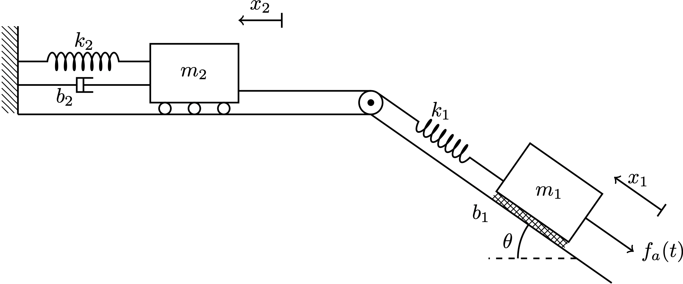
3 Mass hanging on inclined plane
Two masses are connected to each other with an ideal pulley. One of them is on a friction-full inclined plane while the other rests on friction-less wheels. The coordinates \(x_1\) and \(x_2\) are measured relative to some fixed locations, which have been chosen such that when \(x_1 = x_2 = 0\), there is no tension or compression in the springs. A force \(f_a(t)\) is applied to the inclined mass as shown.
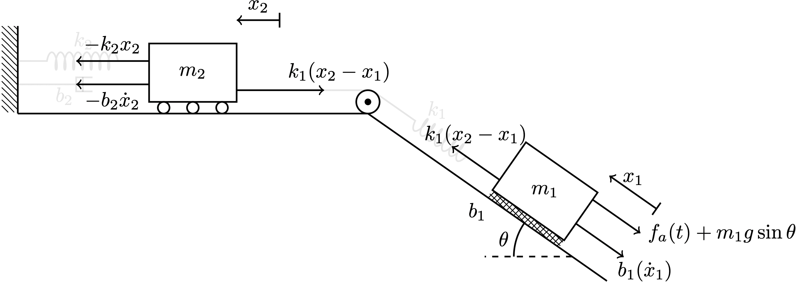
3.1 Free body diagrams
Draw the free body diagrams for this system.
3.2 Governing Equations
Write down two second-order differential equations for the motion of this system.
\[ \begin{aligned} m_2 \ddot{x}_2 &= - k_2 x_2 - b_2 \dot{x}_2 - k_1 (x_2-x_1) \\ m_1 \ddot{x}_1 &= \phantom{- k_2 x_2} -b_1 \dot{x}_1 + k_1(x_2-x_1) - m_1 g \sin \theta - f_a(t) \end{aligned} \]
3.3 Equilibrium value
Under gravity alone (i.e., \(f_a(t) = 0\)), this system won’t naturally stay at \(x_1=x_2=0\). Instead, it will settle to some equilibrium value. Determine mathematical expressions for the equilibrium value of \(x_1\) and of \(x_2\), in terms of the parameters given in the problem and \(g\), the acceleration due to gravity..
The equilibrium value arises from the governing equations in the condition when the system has become stationary.
\[ \begin{aligned} m_2 \cancel{\ddot{x}_2} &= - k_2 x_2 - b_2 \cancel{\dot{x}_2} - k_1 (x_2-x_1) \\ m_1 \cancel{\ddot{x}_1} &= \phantom{- k_2 x_2} -b_1 \cancel{\dot{x}_1} + k_1(x_2-x_1) - m_1 g \sin \theta - \cancel{f_a(t)} \end{aligned} \]
This gives us two equations for \(x_1\) and \(x_2\). \[ \begin{aligned} 0 &= - k_2 x_2 - k_1 (x_2-x_1) \\ 0 &= k_1(x_2-x_1) - m_1 g \sin \theta \end{aligned} \] Adding up these equations, we find that \[-k_2 x_2 - m_1 g \sin \theta = 0 \implies x_2 = \boxed{-\frac{m_1 g}{k_2} \sin \theta}\] and thus, \[{x_1 = \frac{k_2 + k_1}{k_1} x_2} = \boxed{- \frac{k_2 + k_1}{k_1 k_2} m_1 g \sin \theta} \]
The boxed quantities are the equilibrium values of \(x_2\) and \(x_1\).
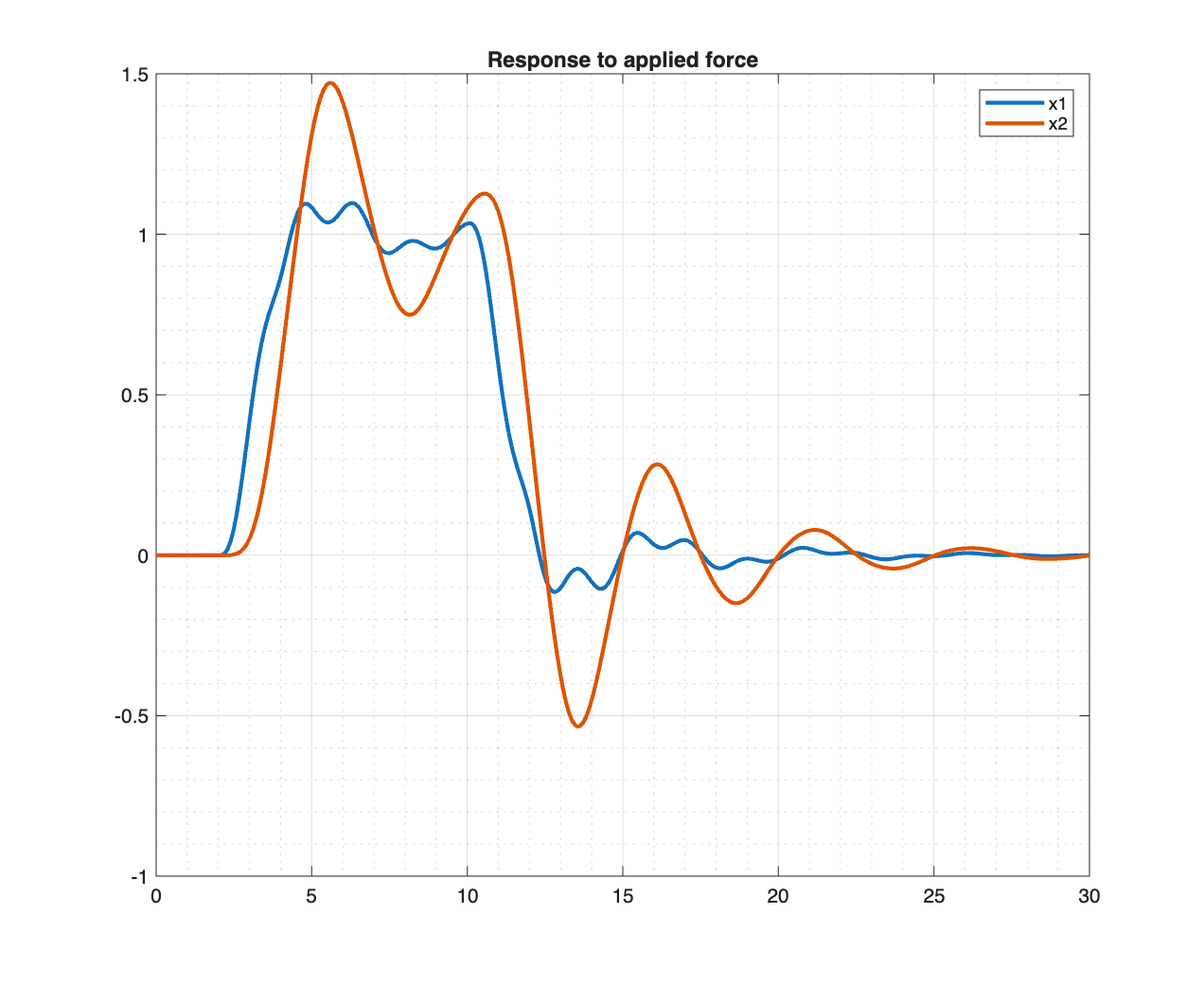
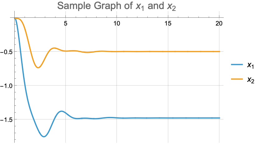
If the system is initialized with \(x_1 = x_2 = \dot{x}_1 = \dot{x}_2 = f_a(t)=0\), the values of \(x_1\) and \(x_2\) follow the graph shown below. The property values used are shown in the table below.
| Parameter | Quantity |
|---|---|
| \(m_1\) | 1 |
| \(m_2\) | 3 |
| \(b_1\) | 2 |
| \(b_2\) | 1 |
| \(k_1\) | 5 |
| \(k_2\) | 10 |
| \(\theta\) | \(30^{\circ}\) |
3.4 Block Diagram
Make a block diagram for this system. In your block diagram, gather the terms related to gravity and the terms related to the applied force \(f_a(t)\) in a single arrow, which you should show as an input to your system.
The block diagram is shown below. It is possible to arrange the information differently.

3.5 Simulink
Get the Simulink file model1.slx, which contains an incomplete simulation of the hanging mass system. Please also place the accompanying files inclinedhang_runsimulink.m and inclinedhang_setupvariables.m in the same folder as your Simulink model file.
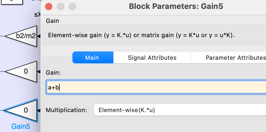
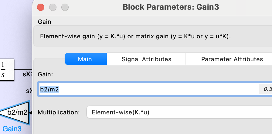
3.5.1 Populate all gain blocks
Most rectangular blocks in a traditional block diagram are indicated in Simulink by triangular ‘gain’ blocks. Determine what goes in each ‘gain’ block. For example, if the sum of two MATLAB variables a+b, enter it like so. Some blocks have been correctly populated for you.
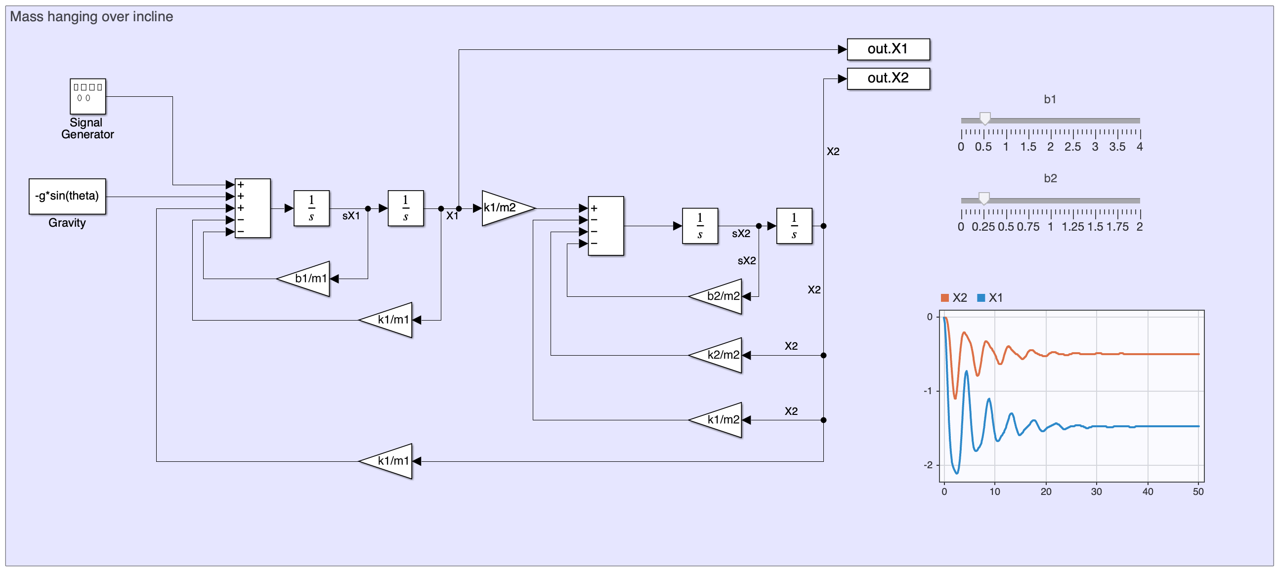
Turn in a screenshot of your completed Simulink diagram.
The completed diagram should look like the following.
3.5.2 Overdamped?
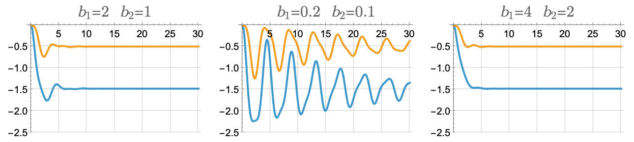
Does the system as a whole seem overdamped, underdamped, or critically damped when you use the highest allowed values of \(b_1=4\) and \(b_2=2\) ? It is sufficient to write a single-word answer to this question.
This system seems underdamped, since there is some oscillation before it settles into a steady-state value, albeit small.
3.5.3 Explore Parameters
While setting the applied force \(f_a(t)\) to zero, set the sliders to different values for \(b_1\) and \(b_2\) between the ranges provided. Select some values for which you see qualitatively different behavior, and save the corresponding plots. There are many ways to do this; you can use inclinedhang_runsimulink.m or you can write your own script. If you’re really having trouble, a screenshot of the “view” panel in Simulink will also suffice.
- Make one set of plots using the values from Table 1. Your graph should look very similar to Figure 1.
- Choose some values of \(b_1\) and \(b_2\) that show more “bouncy-ness” and look qualitatively different from Figure 1.
- Choose some values of \(b_1\) and \(b_2\) that show much less “bouncy-ness”.
For each of the above cases, a plot together with values of \(b_1\) and \(b_2\) (either in the form of a legend/label or as accompanying text) is all you need to turn in. There will be three plots in total, each of them showing both \(x_1\) and \(x_2\).
The following figures were produced using a numerical solution of the governing equations in Mathematica.