Appendix for Final Exam

ENGR 12, Spring 2026.

1 Appendix

1.1 Units

In the SI system,

• The units of resistance are Ohms,
• The units of capacitance are Farads, and
• The units of inductance are Henrys.

Electrical quantities in the base units of kilograms, seconds, meters, and Amperes are not always very useful. However, it is useful to note that:

• Multiplying Ohms by Farads gives seconds, and
• Multiplying Henrys by Farads gives seconds squared.

1.2 First-order systems

A first-order system with transfer function \(\frac{1}{\tau s + 1}\) has time constant \(\tau\). In connection with time constants, the following table may be useful.

The free response of a first-order system \(\tau \dot{x} + x = f(t) = 0\) initialized at \(x=x_0\) at integer multiples of \(\tau\) is given by the following table.

Time	Value	Decimal	Percent
\(t=0 \tau\)	\(x=x_0 e^{-0}\)	\(x=1.0 x_0\)	100%
\(t=1 \tau\)	\(x=x_0 e^{-1}\)	\(x=0.3678x_0\)	36.7%
\(t=2 \tau\)	\(x=x_0 e^{-2}\)	\(x=0.1353 x_0\)	13.5%
\(t=3 \tau\)	\(x=x_0 e^{-3}\)	\(x=0.0497 x_0\)	4.9%
\(t=4 \tau\)	\(x=x_0 e^{-4}\)	\(x=0.0183 x_0\)	1.8%
\(t=5 \tau\)	\(x=x_0 e^{-4}\)	\(x=0.0067 x_0\)	0.6%

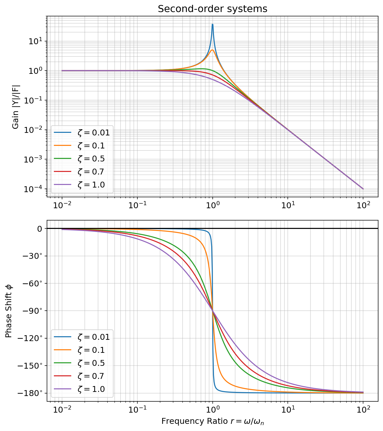
1.3 Second-order systems

The second-order differential equation \(\displaystyle m \ddot{x} + b \dot{x} + kx = f(t)\) can be represented using the transfer function \(\displaystyle \frac{\omega_n^2}{s^2 + 2 \zeta \omega_n s + \omega_n^2}\) if the input is \(f(t)\) and the output \(kx\), where the undamped natural frequency is \[\omega_n = \sqrt{k/m}\] and the damping ratio is \[\zeta = \frac{b}{2 \sqrt{mk}}.\]

The solution to the differential equation \[m \ddot{x} + b \dot{x} + k x = 0\] has three possible forms depending on whether the roots of the characteristic polynomial are:

1. Real and distinct: \(\displaystyle x(t) = c_1 e^{\lambda_1 t} + c_2 e^{\lambda_2 t}\), where \(\lambda_1\) and \(\lambda_2\) are the two roots of the characteristic polynomial
2. Complex: \(\displaystyle x(t) = e^{r t} \left( c_1 \cos \omega_d t + c_2 \sin \omega_d t \right)\) where \(r\) and \(\omega_d\) are the real and imaginary parts of the roots of the characteristic polynomial
3. Real and repeated: \(\displaystyle x(t) = \left(c_1 + c_2 t \right) e^{\lambda t}\) where \(\lambda\) is the repeated root.

For underdamped systems,

• The damped natural frequency is \(\displaystyle \omega_d = \omega_n \sqrt{1-\zeta^2}\)
• The resonant frequency is \(\displaystyle \omega_d = \omega_n \sqrt{1-2\zeta^2}\)
• The time constant is \[\frac{1}{\zeta \omega_n}\]

1.4 Fourier Series

A periodic function \(x(t)\) with period \(P\) is equal to the convergent infinite series

\[ \begin{aligned} x(t) &= a_0 + \sum_{n=1}^{\infty} \left( a_n \cos \left( \frac{2 \pi n t}{P} \right) + b_n \sin \left( \frac{2 \pi n t}{P} \right) \right) \\ x(t) &\approx a_0 + \sum_{n=1}^{N} \left( a_n \cos \left( \frac{2 \pi n t}{P} \right) + b_n \sin \left( \frac{2 \pi n t}{P} \right) \right) \end{aligned} \]

for \(a_n\), \(b_n\) given by the Euler Formulas:

\[ \begin{aligned} a_0 &= \frac{1}{P} \int_{-P/2}^{+P/2} x(t) dt \\ a_n &= \frac{2}{P} \int_{-P/2}^{+P/2} x(t) \cos \left( \frac{2 \pi n t}{P} \right) dt \quad n > 0\\ b_n &= \frac{2}{P} \int_{-P/2}^{+P/2} x(t) \sin \left( \frac{2 \pi n t}{P} \right) dt \quad n > 0\\ \end{aligned} \]

1.5 Bode Plots of Second-order systems

1.6 Partial Fraction Expansion

Consider the rational function \[F(s) = \frac{N(s)}{D(s)} = \frac{b_m s^m + b_{m-1} s^{m-1} + ... + b_0 s^0}{s^n + a_{n-1} s^{n-1} + ... + a_0 s^{0}}\]

1.6.1 Distinct Poles

If \(D(s)\) has \(n\) distinct roots, then we can use partial fractions to expand

\[F(s) = \frac{N(s)}{D(s)} = \frac{A_1}{s-s_1} + \frac{A_2}{s-s_2} + ... + \frac{A_n}{s-s_n}\]

where \[A_i = \lim_{s\rightarrow s_i} \left[ (s-s_i)F(s) \right] \]

1.6.2 Repeated Poles

Let \(F(s)=\frac{N(s)}{D(s)}\) where \(D(s)\) has \(2\) repeated poles and \(n-2\) distinct poles. Then we can use partial fractions to expand

\[F(s) = \frac{N(s)}{D(s)} = \frac{A_{11}}{(s-s_1)^2} + \frac{A_{12}}{s-s_1} + \frac{A_3}{s-s_3} + ... + \frac{A_n}{s-s_n}\]

where the coefficients \(A_3,...A_n\) can be found using a similar process as before: \[A_i = \lim_{s\rightarrow s_i} \left[ (s-s_i)F(s) \right] \]

and we have formulas for the numerators of the repeated poles:

\[A_{11} = \lim_{s\rightarrow s_1} \left[ (s-s_1)^2F(s) \right] \] \[A_{12} = \lim_{s\rightarrow s_1}\left( \frac{d}{ds} \left[ (s-s_1)^2 F(s)\right]\right)\]

1.6.3 Complex Poles

If \(D(s)\) has two complex roots, then \(F(s)\) can be expanded as \[F(s) = \frac{K_1}{s-(r+i\omega)} + \frac{K_2}{s-(r-i\omega)}\] where \(\omega\) is the imaginary part of the complex roots and \(r\) the real part.

\[ \begin{aligned} K_1 &= \lim_{s \rightarrow r+i\omega} \left[ (s-(r+i\omega))F(s) \right] \\ K_2 &= \lim_{s \rightarrow r-i\omega} \left[ (s-(r-i\omega))F(s) \right] \end{aligned} \]

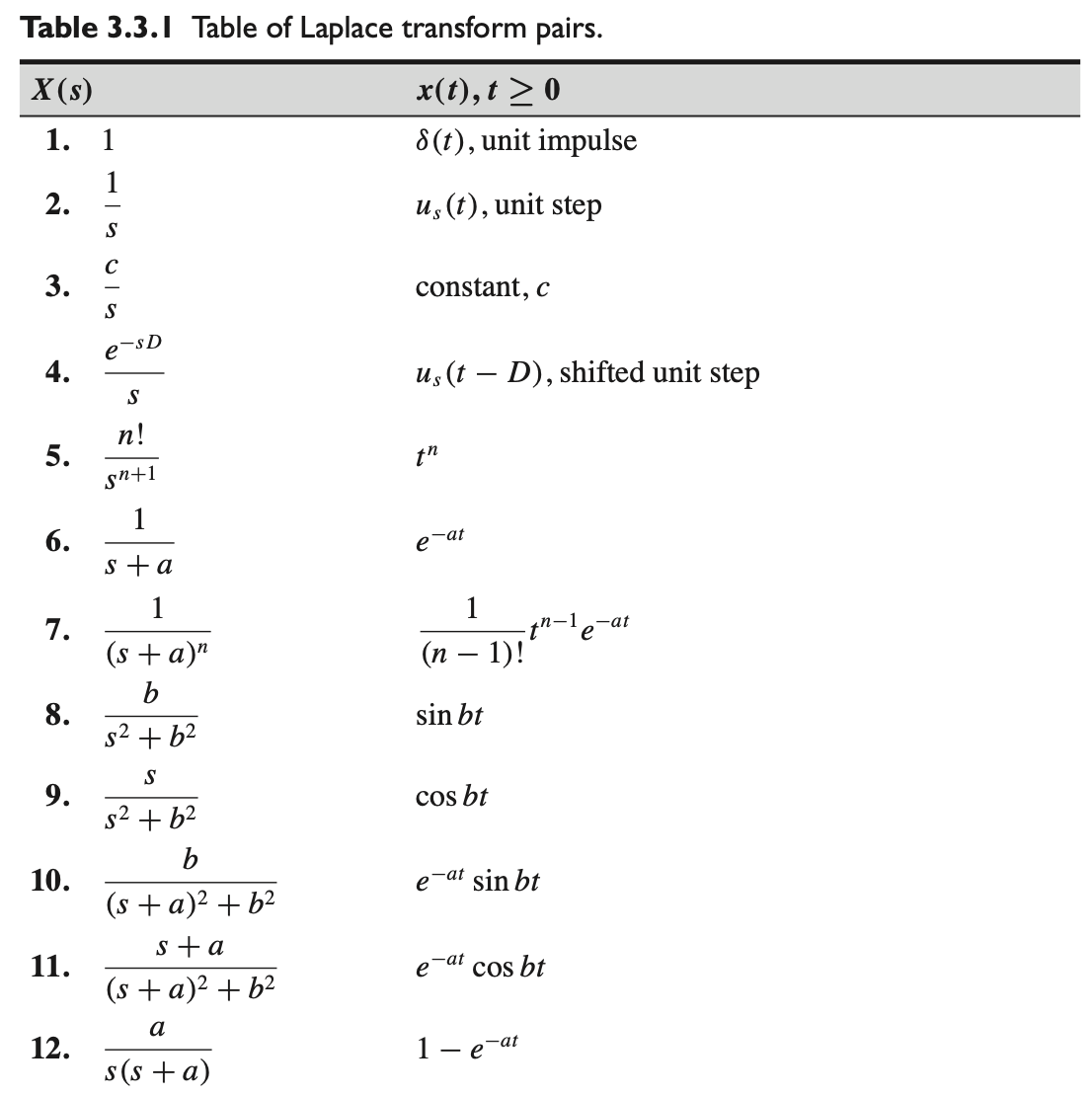
1.7 Laplace Transfroms

The Laplace Transform of a function \(x(t)\) is defined as the following function of \(s\): \[\lim_{T \rightarrow \infty} \int_0^{T} x(t)e^{-st} dt \tag{1}\]

This is a function of \(s\), not a function of \(t\). We give the expression in Equation 1 the name \(X(s)\).

\[X(s) = \boxed{\lim_{T \rightarrow \infty} \int_0^{T} x(t)e^{-st} dt} = \int_0^{\infty} x(t)e^{-st} dt\]

\[x(t) \rightarrow \text{Laplace Transform} \rightarrow X(s) \]

\[x(t) \rightarrow \mathcal{L}[\cdot] \rightarrow X(s)\]

\[\boxed{\mathcal{L}[x(t)] = X(s)}\]

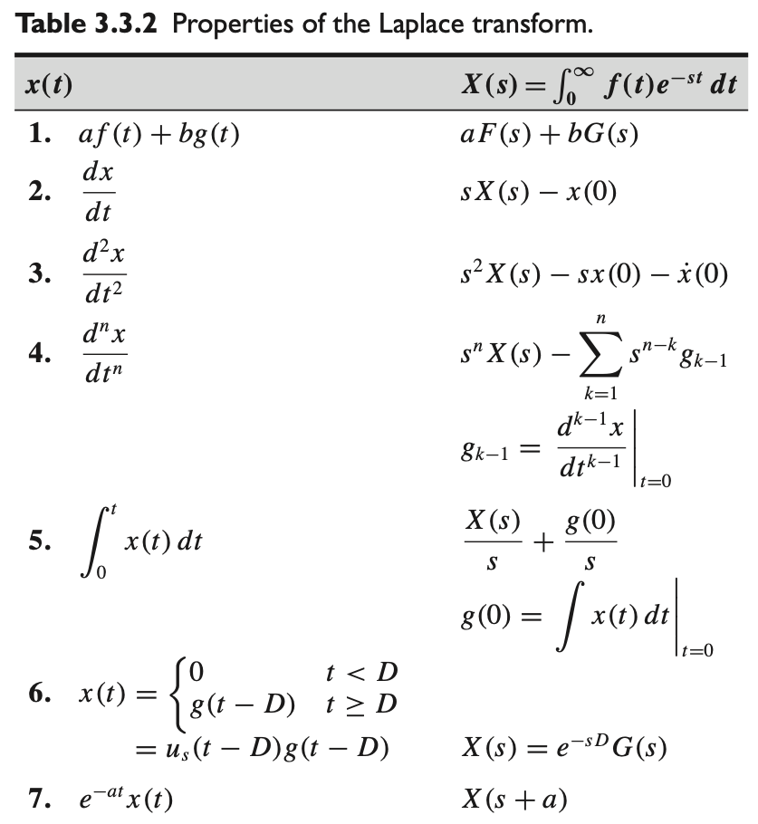
1.8 Laplace Tables