Midterm
ENGR 12, Spring 2026.
| Exam Date | Thu, Mar 19, 2026 |
| Duration | Two hours (120 minutes) |
| # of questions | 8 |
| Approx. time per question | 15 mins |
Instructions
Answer all questions. Each question is equally weighted. You are allowed to use a scientific calculator. On multiple-choice -type questions, full credit will be awarded for making the correct selection, and partial credit may be awarded when wrong selections are accompanied by a partially correct explanation. No external resources may be consulted. An appendix is provided.
1 Coupled vs Uncoupled Linear Equations
We are considering four systems, each of which have two state variables. The governing equation for each of the systems is as follows:
\[\frac{d}{dt} \begin{bmatrix} y_1 \\ y_2 \end{bmatrix} = \underbrace{\begin{bmatrix} a & b \\ c & d \end{bmatrix}}_{A} \begin{bmatrix} y_1 \\ y_2 \end{bmatrix}\]
Here, the matrix \(A\) is called the ‘system matrix’ and expresses compactly how the rate of change of the state variables depends on the state variables themselves.
Each of the four systems has a different system matrix \(A\) as shown in the table below. Match the system to the correct description by drawing lines from the matrix to its correct description. There is exactly one correct description for each matrix.
| No. | System Matrix | Description |
|---|---|---|
| 1 | \(\begin{bmatrix} 3 & 0 \\ 0 & -2 \end{bmatrix}\) | \(y_1\) and \(y_2\) are two-way coupled, i.e., the rate of change of \(y_1\) depends on \(y_2\) and the rate of change of \(y_2\) depends on \(y_1\) |
| 2 | \(\begin{bmatrix} 1 & -1 \\ 0 & -3 \end{bmatrix}\) | \(y_1\) and \(y_2\) are one-way coupled, i.e., the rate of change of \(y_1\) depends on \(y_2\) but the rate of change of \(y_2\) does not depend on \(y_1\) |
| 3 | \(\begin{bmatrix} 2 & -4 \\ -2 & 7 \end{bmatrix}\) | \(y_1\) and \(y_2\) are one-way coupled, i.e., the rate of change of \(y_2\) depends on \(y_1\) but the rate of change of \(y_1\) does not depend on \(y_2\) |
| 4 | \(\begin{bmatrix} 2 & 0 \\ -1 & 3 \end{bmatrix}\) | \(y_1\) and \(y_2\) are uncoupled, i.e., the rate of change of \(y_1\) does not depend on \(y_2\) and the rate of change of \(y_2\) does not depend on \(y_1\) |
Blank page
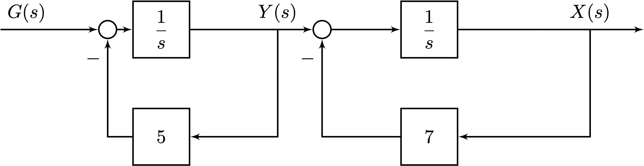
2 Block Diagrams
Consider the block diagram below.
2.1 Simplifying
We would like to simplify this block diagram using the following block diagram:
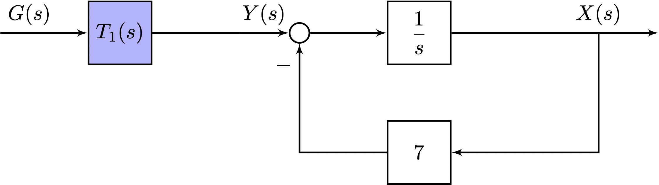
Determine the expression \(T_1(s)\).
2.2 Transfer Function
Determine an expression, in terms of \(s\), for the transfer function between the input \(G(s)\) and the output \(X(s)\).
Blank Page
3 Laplace Transforms
3.1 Converting from frequency domain to time domain.
Given \[F(s) = \frac{1}{s(3s+2)},\] find a mathematical expression for the function \(f(t)\). Show all your work for full credit.
3.2 Converting from time domain to frequency domain
Find the transfer function for a third-order system given by
\[\dddot{x} = 2 \ddot{x} - 4 \dot{x} + 3x + f(t)\]
Blank Page
4 Impulse and Step Functions
4.1 Sketch
A certain system \(a\dot{x} + b x = f(t)\) is subjected to a unit impulse input at time \(t=2\) and a unit step input at time \(t=4\). Make a qualitatively correct sketch of \(f(t)\).
4.2 Relation between impulse and step
Which of the following is true? There may be more than one answer.
Blank Page
5 Inputs
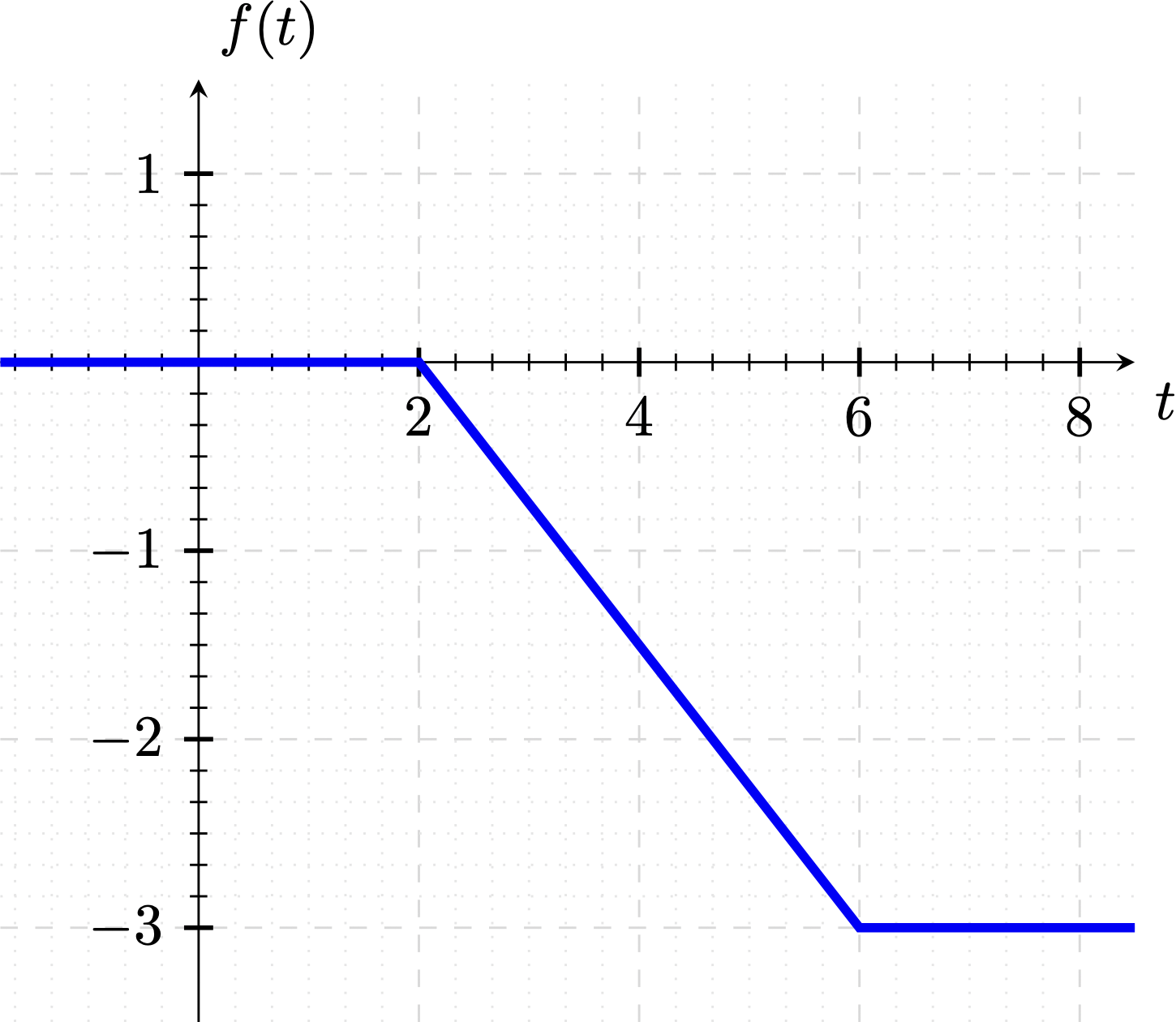
Which of the following is a correct mathematical expression for the function of time shown below? There is only one correct answer.
Blank Page
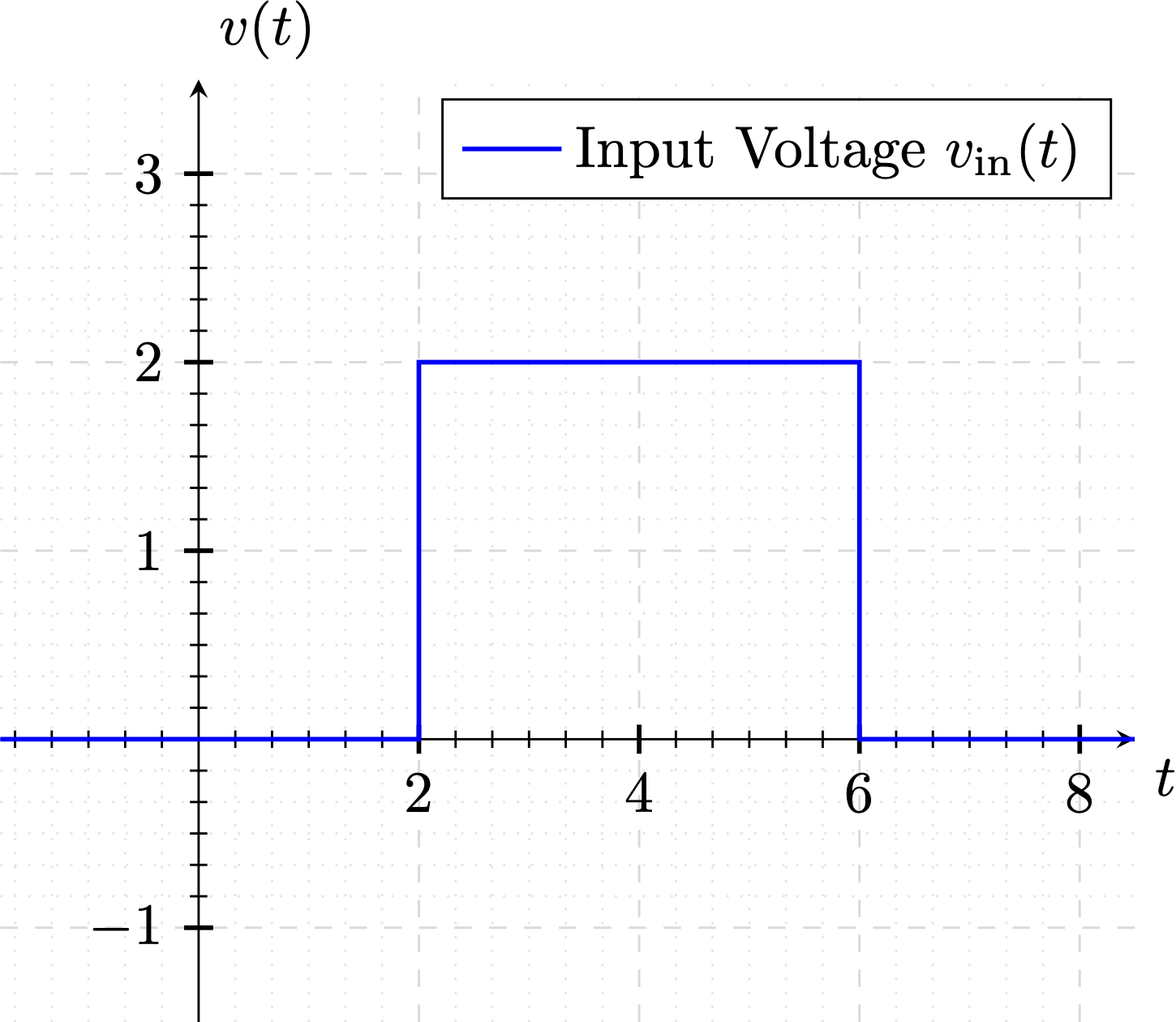
6 ‘Pulse response’

An RC Circuit, shown in Figure 4, has a variable input voltage \(v_{\text{in}}\) given by a ‘pulse’ function \[ v_{\text{in}}(t) = \begin{cases} 0 & t < 2 \\ 2 & 2 \leq t < 6 \\ 0 & t \geq 6. \end{cases} \]
The voltage across the capacitor is initially \(2.0\) Volts.
Sketch a graph of the voltage across the capacitor, \(v_c\), against time for the following cases:
| Case | Resistance | Capacitance |
|---|---|---|
| 1 | \(1.25 \mathrm{M} \Omega\) | \(0.8 \mu F\) |
| 2 | \(1.25 \mathrm{M} \Omega\) | \(0.08 \mu F\) |
using the graphs below.
Blank Page
7 Energy
A spring-mass system is shown below.
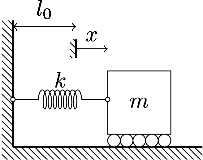
The spring has a rest length of \(l_0\), and the position coordinate \(x\) is defined such that, when \(x=0\), the spring exerts no force in either direction.
This system has the following initial conditions and parameters:
| Quantity | Value |
|---|---|
| Initial Position | \(0\) meters |
| Initial Velocity | \(+2.0\) m/s |
| Spring Constant | \(5\) N/m |
| Mass | \(0.2\) kg |
A graph of the energy in the system as a function of time is shown below.
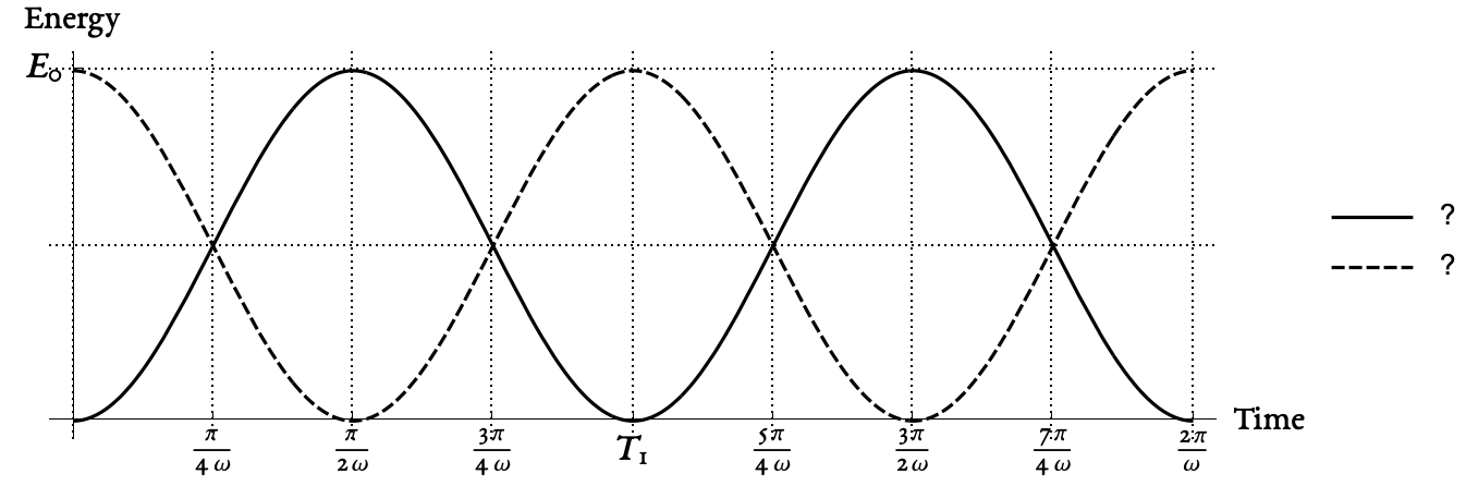
- Label the two lines on the graph with ‘kinetic energy’ and ‘potential energy’.
- Determine numerical values for \(E_0\) and \(T_1\).
Blank Page
8 Second-order systems with damping
A spring-mass damper system has the following differential equation:
\[m \ddot{x} + 2 \dot{x} + 4x = f(t)\]
8.1 Characteristic polynomial
Write down the characteristic polynomial for this system in terms of \(m\) and \(s\).
8.2 Selecting the value of \(m\)
- Write down a value of \(m\) for which the characteristic polynomial of the system will have two distinct negative roots.
- Write down a value of \(m\) for which the characteristic polynomial of the system will have two complex roots with negative real part.
- Suppose the system is initialized with no input \(f\). For what value of \(m\) will the free response of this system die down to zero the quickest?
Blank Page
9 Appendix
9.1 First-order systems
The time constant in a first-order system \[a \dot{x} + b x = f(t)\]is given by the ratio \(a/b\).
9.2 Second-order systems
The second-order differential equation
\[m \ddot{x} + b \dot{x} + kx = 0\]
can be represented by the equation
\[\ddot{x} + 2 \zeta \omega_n x + \omega_n^2 x = 0\]
where the undamped natural frequency is \[\omega_n = \sqrt{k/m}\] and the damping ratio is \[\zeta = \frac{b}{2 \sqrt{mk}}.\]
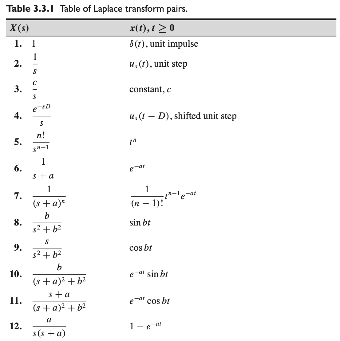
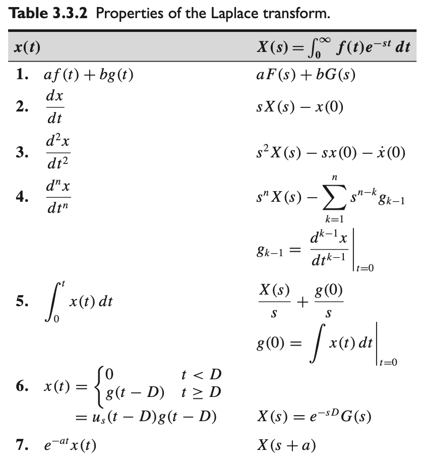
9.3 Laplace Transfroms
The Laplace Transform of a function \(x(t)\) is defined as the following function of \(s\): \[\lim_{T \rightarrow \infty} \int_0^{T} x(t)e^{-st} dt \tag{1}\]
This is a function of \(s\), not a function of \(t\). We give the expression in Equation 1 the name \(X(s)\).
\[X(s) = \boxed{\lim_{T \rightarrow \infty} \int_0^{T} x(t)e^{-st} dt} = \int_0^{\infty} x(t)e^{-st} dt\]
\[x(t) \rightarrow \text{Laplace Transform} \rightarrow X(s) \]
\[x(t) \rightarrow \mathcal{L}[\cdot] \rightarrow X(s)\]
\[\boxed{\mathcal{L}[x(t)] = X(s)}\]
9.4 Laplace Tables