Problem Set 5 Solutions
ENGR 12, Spring 2026.
Solutions
1 Trigonometric and Exponential Representations
We learn that a particular initial value problem has the following solution:
\[x(t) = 2 \cos \left( \omega t + \frac{\pi}{6} \right)\]
Write down this function in the following forms, in each case specifying the numerical value of any constants. For complex numbers, you must state their real and imaginary parts.
- \(A_1 \cos \omega t + A_2 \sin \omega t\), where \(A_1,A_2 \in \mathbb{R}\)
- \(A_3 \sin (\omega t + \phi_3)\), where \(A_3 \in \mathbb{R}\), \(\phi_3 \in [0,2\pi)\)
- \(P_1 e^{i \omega t} + P_2 e^{-i \omega t}\), where \(P_1,P_2 \in \mathbb{C}\)
- \(\mathrm{Re} \left[ A_4 e^{i(\omega t + \phi_4)}\right]\), where \(A_4 \in \mathbb{R}\), \(\phi_4 \in [0,2\pi)\)
- \(\mathrm{Im} \left[ A_5 e^{i(\omega t + \phi_5)}\right]\), where \(A_5 \in \mathbb{R}\), \(\phi_5 \in [0,2\pi)\)
We make use of the identity \(\cos (A+B) = \cos A \cos B - \sin A \sin B\). Then, we have \[ \begin{aligned} 2 \cos \left( \omega t + \pi/6 \right) & \\ &= 2 \cos \omega t \cos \pi/6 - 2 \sin \omega t \sin \pi/6 \\ &= 2 \cdot \frac{\sqrt{3}}{2} \cos \omega t - \frac{2}{2} \sin \omega t \\ &= \boxed{\sqrt{3} \cos \omega t - \sin \omega t} \end{aligned} \]
For this part we notice that sines are just 90-degree-shifted cosines. After a quick sanity check to see which way the shift goes, we can write
\[2 \cos ( \omega t + \pi/6) = 2 \sin ( \omega t + \pi/6 + \pi/2) = \boxed{2 \sin \left(\omega t + \frac{2\pi}{3} \right)} \]
For this part, we make use of the fact that \[\cos \omega t = \frac{1}{2} \left( e^{i \omega t} - e^{-i \omega t} \right).\] The foregoing identity can be derived by using Euler’s formula \(e^{i \theta} = \cos \theta + i \sin \theta\) and we will not derive it. From this starting point, we get \[ \begin{aligned} A \cos \omega t &= \frac{A}{2} \left( e^{i \omega t} - e^{-i \omega t} \right) \\ \implies A \cos (\omega t + \phi) &= \frac{A}{2} \left( e^{i (\omega t + \phi)} - e^{-i (\omega t + \phi)} \right) \\ &= \frac{A}{2} e^{i \phi} e^{i \omega t} + \frac{A}{2} e^{-i \phi} e^{-i\omega t} \end{aligned} \] The number \(\displaystyle \frac{A}{2} e^{i \phi}\) is a complex number with magnitude \(A/2\) and argument \(\phi\). In this case, we are using \(\phi = \pi/6\). We need to use a small amount of trigonometry to decide what this complex number is in \(a+bi\) format, which we won’t explicitly write out. The two complex numbers \(1 e^{i \pi /6}\) and \(1 e^{-i\pi/6}\) are: \(\frac{\sqrt{3}}{2} + \frac{i}{2}\) and \(\frac{\sqrt{3}}{2} i \frac{i}{2}\). Thus, we can write \[2 \cos ( \omega t + \pi/6) = \boxed{\left( \frac{\sqrt{3}}{2} + \frac{i}{2} \right) e^{i \omega t} + \left( \frac{\sqrt{3}}{2} - \frac{i}{2}\right) e^{-i \omega t}} \]
This one’s easy. \[2 \cos ( \omega t + \pi/6) = \boxed{\mathrm{Re} \left[ 2 e^{i (\omega t + \pi/6)} \right]}\]
Since we did part 2, this one’s easy too. We have \[2 \cos ( \omega t + \pi/6) = \boxed{\mathrm{Im} \left[ 2 e^{i (\omega t + 2\pi/3)} \right]}\]
2 Energy Considerations
A spring-mass system is released from rest, i.e., \(\dot{x}(0) = 0\) with position \(x(0) = x_0\), where \(x_0\) is some positive number. The governing equation is \[m \ddot{x} + k x = 0\] and its solution is already known to you.
Assume that \(x\) is defined such that when \(x=0\), the spring is unstretched and uncompressed; it is at its ‘rest length’ and exerts no force. Whenever \(x \neq 0\), the spring exerts a force in the appropriate direction according to Hooke’s Law. Also, whenever \(\dot{x} \neq 0\), the mass possesses a kinetic energy.
The elastic potential energy stored in a spring is \[\frac{1}{2} k x^2. \tag{1}\] The kinetic energy of a moving mass is \[\frac{1}{2} m \dot{x}^2. \tag{2}\]
Use this information to write down a mathematical expression for the elastic potential energy and of the kinetic energy in this spring-mass system, in terms of \(m\), \(k\), \(x_0\) and \(\omega\) that is applicable for any value of time \(t\). Your expression should involve sines and cosines, and not ‘square of sine’/‘square of cosine’.
Also fill in the following table by writing down expressions for each quantity at the respective time.
| Time | Potential Energy | Kinetic Energy |
|---|---|---|
| \(0\) | \(\displaystyle \frac{1}{2} k x_0^2\) | \(0\) |
| \(\displaystyle \frac{\pi}{4 \omega}\) | ||
| \(\displaystyle \frac{\pi}{2 \omega}\) | ||
| \(\displaystyle \frac{3 \pi}{4 \omega}\) | ||
| \(\displaystyle \frac{ \pi}{\omega}\) | ||
| \(\displaystyle \frac{5\pi}{4 \omega}\) | ||
| \(\displaystyle \frac{3\pi}{2\omega}\) | ||
| \(\displaystyle \frac{7 \pi}{4 \omega}\) | ||
| \(\displaystyle \frac{2 \pi}{\omega}\) |
We will make use of the trigonometric identitites \[\begin{aligned} \cos^2 \theta &= \frac{1}{2} \left( 1 + \cos 2 \theta \right) \\ \sin^2 \theta &= \frac{1}{2} \left( 1 - \cos 2 \theta \right) \end{aligned}\]
The motion of the object is described by \[x(t) = x_0 \cos \omega t,\] which we know from Lecture 9. From the definition of the potential energy Equation 1, we can therefore write the potential energy as a function of time using \[ \begin{aligned} \frac{1}{2} k x(t)^2 &= \frac{1}{2} k \left[ x_0^2 \cos^2 \omega t\right] \\ &= \frac{1}{2} k \left[ \frac{1}{2} \left( 1 + \cos(2 \omega t) \right) \right] \\ &= \frac{1}{4} k x_0^2 (1 + \cos( 2 \omega t)) \end{aligned} \]
The velocity \(\dot{x}\) can be found by taking the time derivative of the position. It is \[\dot{x}(t) = - \omega x_0 \sin \omega t.\] From the definition of the kinetic energy Equation 2, we can write the kinetic energy as a function of time using
\[ \begin{aligned} \frac{1}{2} m \dot{x}(t)^2 &= \frac{1}{2} m \left[ (- \omega x_0)^2 \sin^2 \omega t\right] \\ &= \frac{1}{2} m \omega^2 x_0 ^2 \left[ \frac{1}{2} \left( 1 - \cos(2 \omega t) \right) \right] \\ &= \frac{1}{4} m \omega^2 x_0^2 (1 - \cos( 2 \omega t)) \end{aligned} \]
| Time | Potential Energy | Kinetic Energy |
|---|---|---|
| \(0\) | \(\displaystyle \frac{1}{2} k x_0^2\) | \(0\) |
| \(\displaystyle \frac{\pi}{4 \omega}\) | \(\displaystyle \frac{1}{4} k x_0^2\) | \(\displaystyle \frac{1}{4} k x_0^2\) |
| \(\displaystyle \frac{\pi}{2 \omega}\) | \(0\) | \(\displaystyle \frac{1}{2} k x_0^2\) |
| \(\displaystyle \frac{3 \pi}{4 \omega}\) | \(\displaystyle \frac{1}{4} k x_0^2\) | \(\displaystyle \frac{1}{4} k x_0^2\) |
| \(\displaystyle \frac{ \pi}{\omega}\) | \(\displaystyle \frac{1}{2} k x_0^2\) | \(0\) |
| \(\displaystyle \frac{5\pi}{4 \omega}\) | \(\displaystyle \frac{1}{4} k x_0^2\) | \(\displaystyle \frac{1}{4} k x_0^2\) |
| \(\displaystyle \frac{3\pi}{2\omega}\) | \(0\) | \(\displaystyle \frac{1}{2} k x_0^2\) |
| \(\displaystyle \frac{7 \pi}{4 \omega}\) | \(\displaystyle \frac{1}{4} k x_0^2\) | \(\displaystyle \frac{1}{4} k x_0^2\) |
| \(\displaystyle \frac{2 \pi}{\omega}\) | \(\displaystyle \frac{1}{2} k x_0^2\) | \(0\) |
3 Natural Frequency
3.1 Natural Frequency of a pendulum
A pendulum of length \(l\) hanging from a fixed support in Earth’s gravitational field experiences two forces: the force due to gravity and the tension force in the cable.
It is possible to show that the governing equations for the pendulum’s motion are \[l\frac{d^2 \theta}{dt^2} = - g \sin \theta,\] where \(\theta\) is the angle the pendulum makes with the vertical and can be positive or negative as the case may be.
When the pendulum moves a small amount from its equilibrium position of \(\theta = 0\), it has a natural freqency of oscillation that depends on \(g\) and \(l\). Write down a formula for the (angular) natural frequency \(\omega\)$ of a pendulum, and use your formula to calculate how long a pendlum would need to be for it to swing back and forth (i.e. complete one cycle of motion) in exactly 1 second. Give your answer in meters to 4 significant figures.
At small angles \(\theta\), the equation \[l\frac{d^2 \theta}{dt^2} = - g \sin \theta\] can be written as \[l \ddot{\theta} + g \theta = 0\] using the small angle approximation \(\sin \theta \approx \theta\). Dividing through by \(l\), we have \[\ddot{\theta} + \frac{g}{l} \theta = 0,\] which upon comparison with the usual equation for second-order systems with no damping, tells us that the natural frequency is \[\omega = \sqrt{\frac{g}{l}}.\] Earth’s gravitational field is \(g \approx 9.807\) meters per second squared. We would like to choose an angular freqeuncy such that the period, \(T \equiv 1/f\), equals unity. Thus, we need \(omega = 2\pi\) so that \(\omega = 2\pi f \implies 2\pi = 2\pi f \implies f = 1\), i.e., the pendulum’s motion has a freqency of ‘once per second’. Solving the equation \[2\pi = \sqrt{9.807}{l} \implies \boxed{l = 0.2484 \mathrm{ m }}.\]
3.2 Natural Frequency of LC Circuits
An LC circuit with no sources but with some nonzero initial charge across the capacitor is known to have an inductance of \(100 \mathrm{mH}\) (that’s “milli Henry”). What value of capacitance would the capacitor in this circuit need to have such that the voltage across the capacitor changes with a period of \(0.5\) seconds?
We note that the equation \[LC \ddot{v} + v = 0\] is very similar to the equation \[\ddot{x} + \omega^2 x = 0.\] By inspection, we determine that \(\omega^2 = \frac{1}{LC}\). Using the definition of the natural frequency and the period, we can write \[\frac{1}{\sqrt{LC}} = 2\pi f = \frac{2 \pi}{T}.\] We can rearrange this equation to say that the capacitance is \[C = \frac{T^2}{4 \pi^2 L} \implies \boxed{C \approx 63.3 \mathrm{ mF}}.\]
4 Second-order systems in the frequency domain
4.1 Sines and Cosines and their Laplace Transforms
According to the table of Laplace Transforms, \[\mathcal{L}[\cos \omega t] = \frac{s}{s^2+\omega^2}, \quad \mathcal{L}[\sin \omega t] = \frac{\omega}{s^2+\omega^2}.\]
Your task in this question is to show how the above equations are true. Do not use the table of Laplace transforms. Instead, start from the fact that the initial value problem \[ \begin{aligned} \ddot{x} + \omega^2 x &= 0 \\ x(0) &= x_0 \\ \dot{x}(0) &= v_0 \end{aligned} \]
has the solution \[x(t) = x_0 \cos \omega t + \frac{v_0}{\omega} \sin \omega t. \tag{3}\]
This was demonstrated in lecture 9; you do not need to solve an initial value problem to answer this question.
Let us take the Laplace Transform of the given differential equation. We have \[ \begin{aligned} & \mathcal{L}\left[ \ddot{x} + \omega^2 x \right] = 0 \\ &= \mathcal{L}[ \ddot{x}] + \omega^2 \mathcal{L}[x] \\ &= s(sX(s) - x(0)) - \dot{x}(0) + \omega^2 X \\ &= s(sX(s) - x_0) - v_0 + \omega^2 X \\ &= s^2 X - s x_0 - v_0 + \omega^2 X = 0 \end{aligned} \]
Laplace Transform of Cosine
Now, first let’s consider the case when there is some initial \(x(t)\), but zero initial \(\dot{x}(t)\), i.e., \(v_0 = 0\) and \(x_0 \neq 0\). Then, in this case, the solution in the time domain would be Equation 3 with \(v_0=0\), i.e., \[x(t) = x_0 \cos \omega t. \tag{4}\] In the frequency domain, we don’t yet know what \(X(s)\) would be in this case (because we’re not allowed to look at the table of Laplace Transforms), but we do know that \[ \begin{aligned} s^2 X - s x_0 - \cancel{v_0} + \omega^2 X &= 0 \\ \implies (s^2 + \omega^2)X &= s x_0 \\ \end{aligned} \] which means that \[X(s) = x_0 \frac{s}{s^2 + \omega^2} \tag{5}\]
Now, comparing Equation 4 with Equation 5, we can see that if we take the Laplace Transform of Equation 4, we get \[\begin{aligned} \mathcal{L}[x(t)] = \mathcal{L}[x_0 \cos \omega t] \\ X(s) = x_0 \mathcal{L}[\cos \omega t]\end{aligned}\] and, by comparing this with Equation 5, we can say that \[\mathcal{L}[\cos \omega t] = \frac{s}{s^2+\omega^2}, \qquad \text{Q.E.D.}\]
Laplace Transform of Sine
Next, let’s consider the case when there is some initial \(\dot{x}(t)\), but zero initial \({x}(t)\), i.e., \(v_0 \neq 0\) and \(x_0 = 0\). Then, in this case, the solution in the time domain would be Equation 3 with \(x_0=0\), i.e., \[x(t) = \frac{v_0}{\omega} \sin \omega t. \tag{6}\] In the frequency domain, we don’t yet know what \(X(s)\) would be in this case (because we’re not allowed to look at the table of Laplace Transforms), but we do know that \[ \begin{aligned} s^2 X - s \cancel{x_0} - {v_0} + \omega^2 X &= 0 \\ \implies (s^2 + \omega^2)X &= v_0 \\ \end{aligned} \] which means that \[X(s) = \frac{v_0}{s^2 + \omega^2} \tag{7}\]
Now, comparing Equation 6 with Equation 7, we can see that if we take the Laplace Transform of Equation 6, we get \[\begin{aligned} \mathcal{L}[x(t)] = \mathcal{L}[\frac{v_0}{\omega} \sin \omega t] \\ X(s) = \frac{v_0}{\omega} \mathcal{L}[\sin \omega t].\end{aligned} \tag{8}\] Note also that we can write Equation 7 in a more friendly form by writing the equivalent expression \[X(s) = \frac{v_0}{\omega} \frac{\omega}{s^2+\omega^2}.\] By comparing this with Equation 8, we can say that \[\mathcal{L}[\sin \omega t] = \frac{\omega}{s^2+\omega^2}, \qquad \text{Q.E.D.}\]
4.2 Step Response of second-order system
Use Laplace Transforms to determine the response of the second-order system \[\ddot{x} + \omega^2 x = f(t)\] to the forcing function \(f(t) = u_s(t)\), the unit step function. Write down the response as a function of \(s\) and as a function of \(t\). Use the table of Laplace Transforms as needed.
Taking the Laplace Transform of the equation, and ignoring any initial conditions since we are concerned with the response to a forcing function, not the ‘free response’, at the moment, we find \[X(s) = \frac{F(s)}{s^2 + \omega^2}.\] Now, \(F(s)\) is the Laplace Transform of \(f(t) = u_s(t)\), which is \(1/s\). So we have \[X(s) = \frac{1}{s} \frac{1}{s^2 + \omega^2} = \frac{A}{s} + \frac{B}{ss+ i \omega} + \frac{C}{s - i \omega}.\] Equating coefficients of the numerator in the following equation, \[\frac{1}{s(s^2+\omega^2)} = \frac{A}{s} + \frac{B}{s+ i \omega} + \frac{C}{s-i \omega},\] we find that \[ \begin{aligned} 1 &= A(s^2 + \omega^2) + B s (s - i \omega) + Cs(s+i\omega) \\ \implies A + B + C &= 0 \\ i \omega C - i \omega B &= 0 \implies C = B. \\ A \omega^2 &= 1 \implies A = \frac{1}{\omega^2} \\ \frac{1}{\omega^2} + 2B &= 0 \implies B = -\frac{1}{2 \omega^2} \implies C = -\frac{1}{2 \omega^2}. \end{aligned} \]
So the step response can be written as the sum of the following fractions:
\[X(s) = \frac{1/\omega^2}{s} + \frac{-1/(2 \omega^2)}{s+i \omega} + \frac{-1/(2\omega^2)}{s - i \omega}\]
For the time domain, we can take the inverse Laplace Transform of the above, and we find \[ \begin{aligned} x(t) &= \frac{1}{\omega^2} - \frac{1}{2\omega^2} \left( e^{i \omega t} + e^{-i \omega t}\right) \\ &= \frac{1}{\omega^2} - \frac{1}{\omega^2} \cos \omega t \end{aligned}\]
The first time represents a constant upward shift; the second term represents a cosine function with a negative sign.
5 Simulink
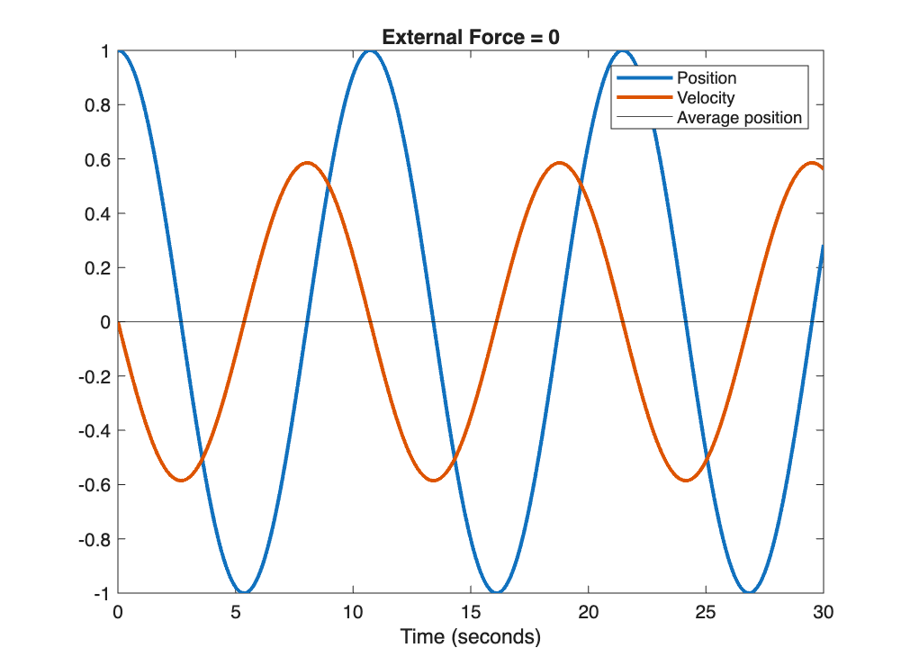
The Simulink model from Lecture 10 can be used to model the behavior of the system \[ m \ddot{x} + k x = f(t),\] with \(f\) taking on many forms. When \(f=0\), Simulink and MATLAB can be used together to generate the following plot.
The code to do so is included below.
% Run Model in Simulink and obtain "out" in Workspace.
out = sim("secondorder1.slx");

figure(1); clf;
plot(out.position,"LineWidth",2);
hold on;
plot(out.velocity,"LineWidth",2);
yline(0,"Color","Black");
legend(["Position","Velocity","Average position"])
title("External Force = 0")
ylabel("")
saveas(gcf,"filename.png")
Generate a plot similar to the above for each of the following cases using MATLAB. The plot should show position, velocity, and a horizontal line for the average position. It should go from \(t=0\) to \(t=30\) and the time-step should be sufficiently small to produce smooth graphs. For each case, turn in the following three items:
- The plot as an image
- Syntax-highlighted MATLAB code showing how you produced it.
- A screenshot of the Simulink model
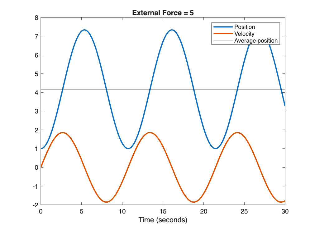
- For the system \[m \ddot{x} + k x = f(t), \quad x(0) = 1, \dot{x}(0) = 0\] set \(m=3.5\), \(k=1.2\) and \(f(t) = 5.0\), i.e., a forcing function that is constant.
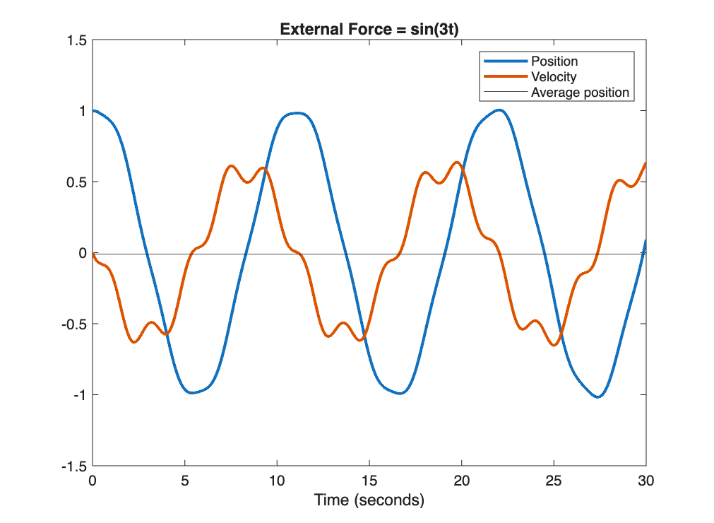
- For the system \[m \ddot{x} + k x = f(t), \quad x(0) = 1, \dot{x}(0) = 0\] set \(m=3.5\), \(k=1.2\) and \(f(t) = sin(3t)\), i.e., a forcing function in which the amplitude is 1 and the angular frequency is 3.
The following MATLAB code was used
%% Case when f(t) = 5.0

% Run Model in Simulink and obtain "out" in Workspace.
out = sim("secondorder1.slx");

figure(2); clf;
plot(out.position,"LineWidth",2);
hold on;
plot(out.velocity,"LineWidth",2);

% Average position:
% Initial value + (max - min)/2
ave = out.position.Data(1) +(max(out.position) - min(out.position))/2;

yline(ave,"Color","Black");
legend(["Position","Velocity","Average position"])
title("External Force = 5")
ylabel("")
saveas(gcf,"f5.png")

%% Case when f(t) = sin(3t)

% Run Model in Simulink and obtain "out" in Workspace.
out = sim("secondorder2.slx");

figure(3); clf;
plot(out.position,"LineWidth",2);
hold on;
plot(out.velocity,"LineWidth",2);

% Average position: seems to be about zero
ave = out.position.Data(1) - (max(out.position) - min(out.position))/2;

yline(ave,"Color","Black");
legend(["Position","Velocity","Average position"])
title("External Force = sin(3t)")
ylabel("")
saveas(gcf,"fsine.png")
The Simulink files used are shown below
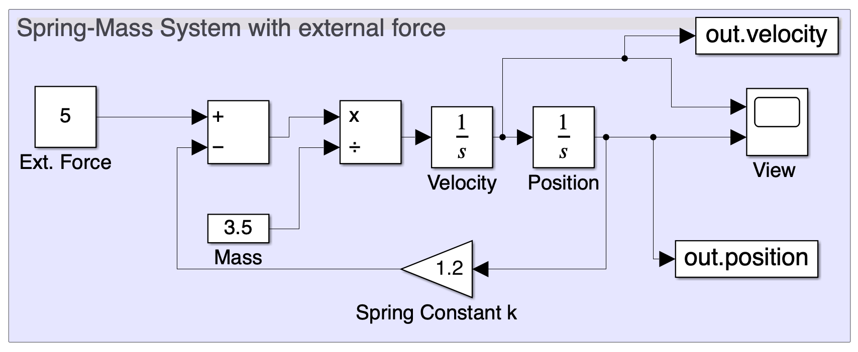
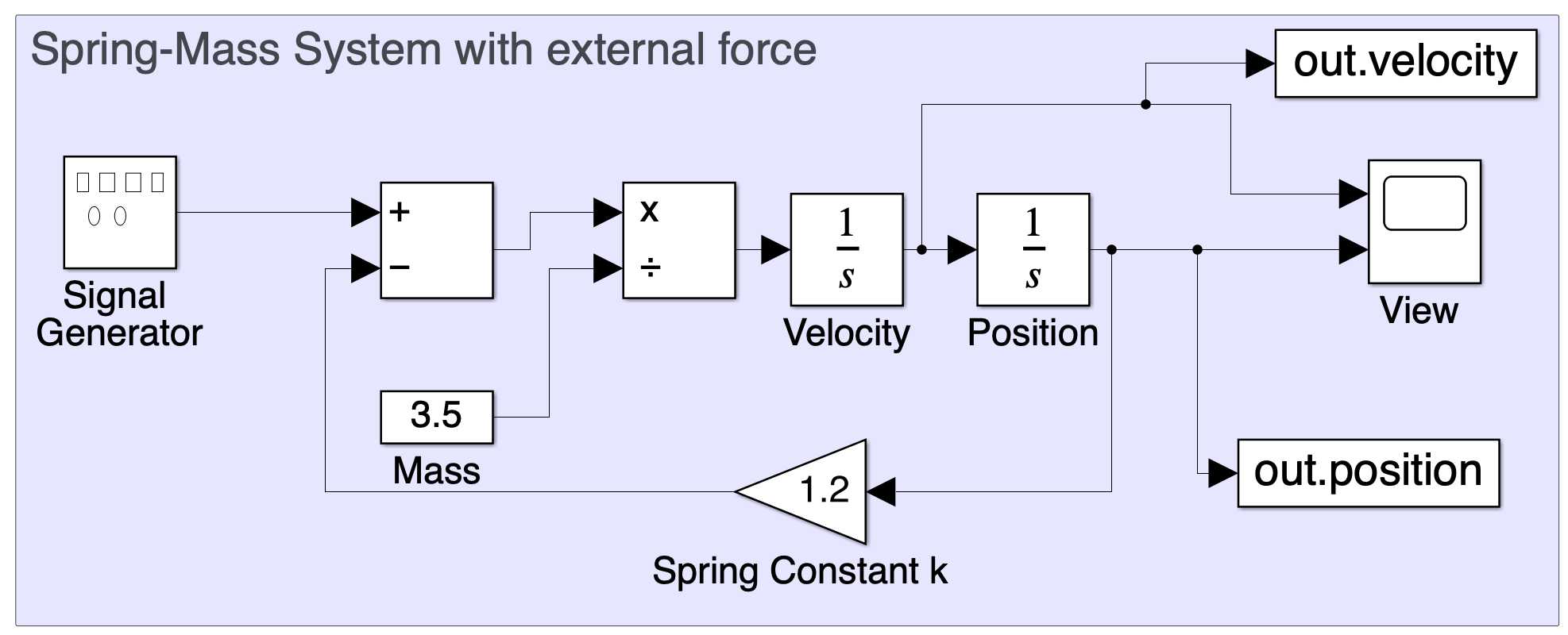
and can be downloaded here and here.
The resulting figures are: