High quality figures for E12

Figures in E12

You will often need to convey the results of your analysis using figures. This page contains examples of code that can be re-used to produce ‘professional’ figures for use in your homework assignments and lab projects.

Why care about high-quality figures?

As an engineer, you will often communicate the results of your design and analysis activities in the form of figures.

Policies on collaboration and attribution

It is okay to re-use code that formats figures in the way that you want. If your friend has made a beautiful figure that you really like, it is sometimes acceptable to reuse the portion of your friend’s code that formats their figures.

The important thing is that you should know how to produce good figures, and this is a skill that you will hone over time as you learn about the capabilities of different programs.

MATLAB

Save the following functions as separate MATLAB files whose file name should be f1.m and f2.m respectively.

function output = f1(x)
% This function takes as input a value of x and returns the value of f(x) =
% x^2 - 3x + 1. It does so using MATLAB's 'vectorized' syntax by placing a
% dot before each operation to indicate it should apply to a whole 'array',
% or 'vector', of numbers.
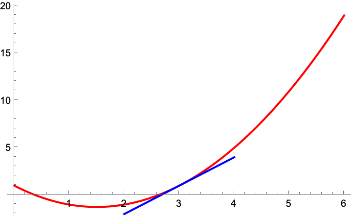
    output = x.^2 - 3.*x + 1;
end

function output = f2(x,m,b)
% This function takes as input a value of x and returns the value of f(x) =
% m*x + b. It does so using MATLAB's 'vectorized' syntax by placing a
% dot before each operation to indicate it should apply to a whole 'array',
% or 'vector', of numbers.
    output = m.*x + b;
end

Then, use the following script to generate a plot. The script can have any file name, but it must be in the same directory as the other two files.

% Pre-compute the values of f1
x = linspace(0,6,100);
y = f1(x);

% Plot the function f1(x) = x^2 - 3x + 1
clf;
plot(x, y,LineWidth=2,Color="r");
hold on;

% Plot the function f2(x,m,b) = m*x + b
% where b and m are given. 
% Do this over a different range of x,
% from 2 to 4
x2 = linspace(2,4,10);

m1 = 3; % Example slope
b1 = -8; % Example y-intercept

plot(x2, f2(x2,m1,b1),"LineStyle","-",Color="b"); % compute f1 on the fly

xlabel('x',FontSize=14);
ylabel('f(x)',FontSize=14);
title('Plot of f1(x)',FontSize=16);
grid on;

Alternatively, you can use MATLAB’s ‘anonymous functions’ to circumvent the need for separate files.

% Define x domain and function
x1 = linspace(0,6,100);
f1 = @(x) x.^2 -3*x + 1;

x2 = linspace(2,4,10);
f2 = @(x,m,b) m .* x + b;

m1 = 3; % Example slope
b1 = -8; % Example y-intercept

% Calculate and plot
plot(x1,f1(x1),'r-',x2,f2(x2,m1,b1),'b--');

% Format the plot better
xlabel('x',FontSize=14);
ylabel('f(x)',FontSize=14);
title('Plot of f1(x)',FontSize=16);
grid on;

% Save it
saveas(gcf,"sample_figure.png");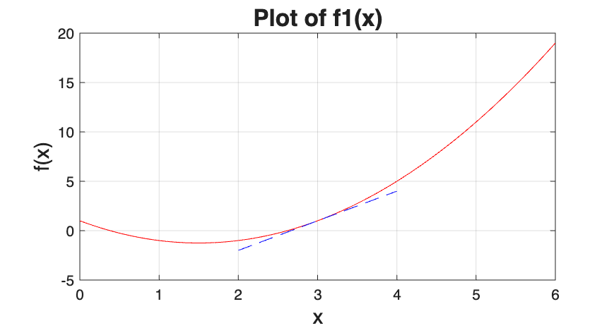

Python

import numpy as np
import matplotlib.pyplot as plt

# Define the functions to be plotted
def f1(x):
    return x**2 - 3*x + 1

def f2(x,m,b):
    return m*x + b

# Define the parabolic function for plotting
x = np.linspace(0,6,100)
y = f1(x)

# Define the straight line
m1 = 3
b1 = -8
x2 = np.linspace(2,4,10)
y2 = f2(x2,m1,b1)

# Make the plots
plt.plot(x,y,'-',x2,y2,'-')
plt.xlabel("x",fontsize=14)
plt.ylabel("f(x)",fontsize=14)
plt.show()

Mathematica

You could also do this in Mathematica as follows

With[{m = 3, b = -8},
 Show[
  Plot[x^2 - 3 x + 1, {x, 0, 6}, PlotStyle -> Red],
  Plot[m x + b, {x, 2, 4}, PlotStyle -> Blue]
  ]
 ]
Export[NotebookDirectory[] <> "plot_example.png", %]