Lecture 12
E12 Linear Physical Systems Analysis
Choice of State Variables is not unique
Consider \(m\ddot{x} + kx = 0\).
One choice of state variables is \(x\) and \(\dot{x}\), position and velocity. \[ \frac{d}{dt} \begin{bmatrix} x \\ \dot{x} \end{bmatrix} = \begin{bmatrix} \dot{x} \\ -(k/m)x \end{bmatrix} = \begin{bmatrix} 0 & 1 \\ -k/m & 0 \end{bmatrix} \begin{bmatrix} x \\ \dot{x} \end{bmatrix} \]
Another choice of state variables is \(x\) and \(m \dot{x}\), position and momentum. What would the above equations be with these as the state variables instead? \[ \frac{d}{dt} \begin{bmatrix} x \\ m\dot{x} \end{bmatrix} = \begin{bmatrix} ? \\ ? \end{bmatrix} = \begin{bmatrix} ? & ? \\ ? & ? \end{bmatrix} \begin{bmatrix} x \\ m\dot{x} \end{bmatrix} \]
\[ \frac{d}{dt} \begin{bmatrix} x \\ m\dot{x} \end{bmatrix} = \begin{bmatrix} \dot{x} \\m \ddot{x} \end{bmatrix} = \begin{bmatrix} \dot{x} \\ - k x \end{bmatrix} = \begin{bmatrix} 0 & 1/m \\ -k & 0 \end{bmatrix} \begin{bmatrix} x \\ m\dot{x} \end{bmatrix} \]
The rest length of a spring and state variables
The rest length \(l_0\) of a spring is the length at which it exerts no force. It’s neither compressed nor extended.
Note: Our springs are always ‘bidirectional’:
- if extended, they pull back;
- if compressed, they push back.
- when their length equals \(l_0\), they don’t push or pull
Measuring the length from the wall

Write down Newton’s 2nd Law for this mass (FBD)
\[m \ddot{x} = f - k (x-l_0)\] \[m \ddot{x} + kx = f + k l_0 \] Let’s say \(f=0\)
The term \(k l_0\) acts like a constant force, i.e., like a step function input
Measuring the length relative to \(l_0\)
\[m \ddot{x} = f - k (x-l_0)\] \[m \ddot{x} + kx = f + k l_0 \]
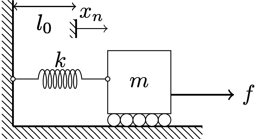
\[x_n = x - l_0\] \[\ddot{x}_n = \ddot{x}\] \[m \ddot{x}_n = f - k x_n\] \[m \ddot{x}_n + kx_n = f\]
- We will often re-define our coordinates \(x\) to get rid of \(l_0\) in our equations.
A note about the ‘order’ of a system
We use the word ‘order’ to refer to two different things.
- A ‘second order equation’ \[\ddot{x} = f(x,\dot{x},t)\]
- A system of two first order equations \[ \dot{x}_1 = f_1(x_1,x_2,t) \\ \dot{x}_2 = f_2(x_1,x_2,t)\]
- Both of these are ‘second order’
- If using block diagrams, you will use two \(\frac{1}{s}\) blocks for each system above
Deciphering the order of a system

What is the order of this system?
Approach 1
Draw free-body diagrams for both systems and write Newton’s laws for each
Approach 2
Count the number of energy-storing elements
\[ \begin{aligned} m_1 \ddot{x}_1 &= \phantom{-}k(x_2-x_1 - l_0) \\ m_2 \ddot{x}_2 &= -k(x_2-x_1-l_0) \\ \end{aligned} \]
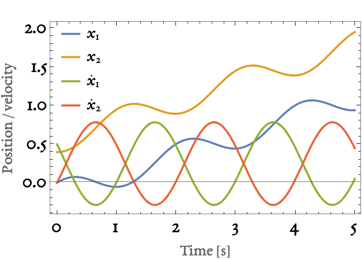
A coupled second-order system in action
\[ \begin{aligned} m_1 \ddot{x}_1 &= \phantom{-}k(x_2-x_1 - l_0) \\ m_2 \ddot{x}_2 &= -k(x_2-x_1-l_0) \\ x_1(0) &= 0, \dot{x}_1(0) = 0.5, x_2(0) = 0.4, \dot{x}_2(0) = 0 \\ m_1 &= m_2 = 1, k = 5, l_0 = 0.7 \end{aligned} \]
Using ode45 to model higher-order systems
2nd order, no forcing
MATLAB’s ode45 can be used to model second-order systems
\[m \ddot{x} + k x = 0 \implies \ddot{x} = -\frac{k}{m} x\]
function dydt = rhs(t,y)
% Implements the right-hand-side of the equation
% dy/dt = f(y,t)
% where y is a vector containing n state variables.
% Here, we are interested in the equation m x'' + k x = 0
% So y1 = x and y2 = x'.
    % un-pack contents of y
    y1 = y(1);
    y2 = y(2);

    % define constants
    k = 5; m = 3;

    % Define what dy/dt is
    dy1dt = y2;
    dy2dt = -(k/m)*y1;

    % Assemble contents of dy/dt into a column vector
    dydt = [dy1dt;dy2dt];
end
Using ode45 to model higher-order systems
2nd order, with forcing
If the function includes an input, MATLAB expects to incorporate this into the ‘right-hand side function’.
- For example, if we have \[m \ddot{x} + k x = f(t) \implies \ddot{x} = -\frac{k}{m}x + f(t) \]
function dydt = rhs(t,y)
% Implements the right-hand-side of the equation
% dy/dt = f(y,t)
% where y is a vector containing n state variables.
% Here, we are interested in the equation m x'' + k x = cos(2t)
% So y1 = x and y2 = x'.
    % un-pack contents of y
    y1 = y(1);
    y2 = y(2);

    % define constants
    k = 5; m = 3;

    % Define what dy/dt is
    dy1dt = y2;
    dy2dt = -(k/m)*y1 + cos(2*t);

    % Assemble contents of dy/dt into a column vector
    dydt = [dy1dt;dy2dt];
end
How to use ode45
- In this class, you will usually not have to write code from scratch.
- Please freely copy, re-use, and modify the code provided in class
- Building an intuition for how to use
ode45takes time.
% Use ode45 from t = 0 to t = 10. Initial conditions are
% x(0) = 1, x'(0) = 0
[t,ysol] = ode45(@rhs,[0,10],[1;0]);

% Make plot in one go
plot(t,ysol); % Plots both columns of 'ysol' in one go

% Make plot in n steps, where n = number of state variables
plot(t,ysol); % Plots both columns of 'ysol' in one go
legend("x","x dot","Location","southeast");
Applying ode45 to spring-mass system
In-class activity: For each of the following scenarios, use MATLAB to plot graphs of position and velocity.
- A spring-mass system is started from rest with a non-zero position. No force is applied.
- A spring-mass system is subjected to a force \(\cos 2t\), starting from rest and the equilibrium position
- A spring-mass system is subjected to the ‘hat’ function from HW 4
Download code from Website > Resources > Numerically Solving Initial Value Problems > Higher Order https://emadmasroor.github.io/E12-S26/Resources/numsol/higherorder
Two coupled spring-mass systems
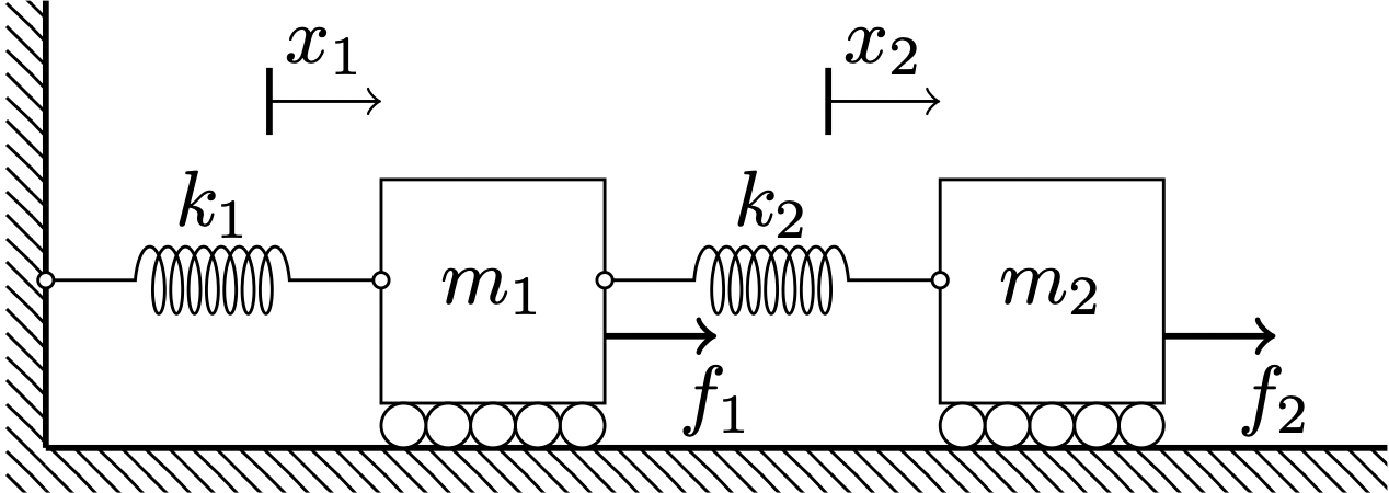
- We define \(x_1\) such that when \(x_1=0\), spring \(k_1\) is at rest length.
- We define \(x_2\) such that when \(x_1 = x_2 = 0\), spring \(k_2\) is at rest length.
Governing equations for two coupled spring-mass systems
\[ \frac{d}{dt} \begin{bmatrix} y_1 \\ y_2 \\ y_3 \\ y_4 \end{bmatrix} = \begin{bmatrix} 0 & 1 & 0 & 0 \\ -(k_1+k_2)/m_1 & 0 & k_2/m_1 & 0 \\ 0 & 0 & 0 & 1 \\ k_2/m_2 & 0 & -k_2/m_2 & 0 \end{bmatrix} \begin{bmatrix} y_1 \\ y_2 \\ y_3 \\ y_4 \end{bmatrix} + \begin{bmatrix} 0 \\ f_1/m_1 \\ 0 \\ f_2/m_2 \end{bmatrix} \]
- This can also be written, with \(n=4\) (the number of state variables): \[\dot{\boldsymbol{y}} = \boldsymbol{A} \boldsymbol{y} + \boldsymbol{b}\]
- \(\boldsymbol{y}\) is of size \(n \times 1\)
- \(\boldsymbol{b}\) is of size \(n \times 1\)
- \(\boldsymbol{A}\) is of size \(n \times n\)
Multiple Input Functions
- A system with n state variables can have m inputs, where \(n\) and \(m\) are any natural numbers.
- A systematic way of treating multiple-input equations is needed
- Consider the last term from before \[ \frac{d}{dt} \begin{bmatrix} y_1 \\ y_2 \\ y_3 \\ y_4 \end{bmatrix} = \begin{bmatrix} 0 & 1 & 0 & 0 \\ -(k_1+k_2)/m_1 & 0 & k_2/m_1 & 0 \\ 0 & 0 & 0 & 1 \\ k_2/m_2 & 0 & -k_2/m_2 & 0 \end{bmatrix} \begin{bmatrix} y_1 \\ y_2 \\ y_3 \\ y_4 \end{bmatrix} + \color{red}{\begin{bmatrix} 0 \\ f_1/m_1 \\ 0 \\ f_2/m_2 \end{bmatrix}} \tag{1}\]
- Collect the \(m\) inputs into an input vector of size \(m \times 1\): \[\boldsymbol{u} = \begin{bmatrix} f_1 \\ f_2 \end{bmatrix}\]
- Define a control matrix \(\boldsymbol{B}\) of size \(n \times m\) such that \(\boldsymbol{B} \boldsymbol{u} =\) the last term in Equation 1.
- Recall that when a matrix of size \(\color{blue}{p} \times \color{brown}{q}\) multiplies a matrix of size \(\color{brown}{q} \times \color{green}{r}\), you get a matrix of size \(\color{blue}{p} \times \color{green}{r}\) \[ \boldsymbol{B} = \begin{bmatrix} 0 & 0 \\ 1/m_1 & 0 \\ 0 & 0 \\ 0 & 1/m_2 \end{bmatrix} \implies \underbrace{{\color{magenta}{\begin{bmatrix} 0 & 0 \\ 1/m_1 & 0 \\ 0 & 0 \\ 0 & 1/m_2 \end{bmatrix}}}}_{\boldsymbol{B}} \begin{bmatrix} f_1 \\ f_2 \end{bmatrix} = \color{red}{\begin{bmatrix} 0 \\ f_1/m_1 \\ 0 \\ f_2/m_2 \end{bmatrix}} \]
- \(B\) has to be constructed by inspection.
Governing equations of a system with multiple inputs
\[\dot{\boldsymbol{y}} = \boldsymbol{A} \boldsymbol{y} + \boldsymbol{B} \boldsymbol{u}\]
- \(\boldsymbol{y}\) is the state vector (\(n \times 1\))
- \(\boldsymbol{A}\) is the system matrix (\(n \times n\))
- \(\boldsymbol{B}\) is the control matrix (\(n \times m\))
- \(\boldsymbol{u}\) is the input vector (\(m \times 1\))
Note:
- Multiplying a matrix with a matrix is the same thing as a dot product
- A ‘(column) vector’ is the same as a ‘matrix with with 1 column’
- To correctly multiply \(A B\), a.k.a. \(A \cdot B\), the number of columns of \(A\) must equal the number of rows of \(B\)
- Matrix multiplication is not commutative, \(A \cdot B \neq B \cdot A\)