Problem Set 4

ENGR 12, Spring 2026.

Due Date	Thu, Feb 19, 2026
Turn in link	Gradescope
URL	`emadmasroor.github.io/E12-S26/Homework/HW4`

Points Distribution

Please note that each of the following grade items is a single rubric item. Each rubric item is scored on a four-level scale of 3-2-1-0. You may wish to take this into account when deciding how to allocate your efforts to each problem.

Problem	Part	% Weightage
Problem 1		20
Problem 2		20
Problem 3		20
Problem 4	4.1	20
Problem 4	4.2	20

1 The top-hat response

In this question we are interested in the response of an RC circuit to a ‘top-hat input’, i.e., an input function \(v_{\text{in}}(t)\) that looks like the top-hat function introduced in Lecture 7. We will proceed with a numerical approach.

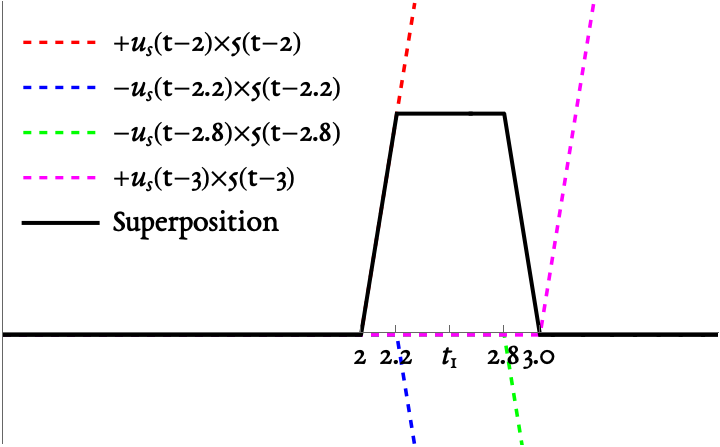
An RC circuit is powered by a voltage source that operates with the function \(f(t)\), where the function \(f(t)\) is given by the figure above, which is the superposition (a fancy word for ‘sum’) of the four shifted-and-rescaled ramp functions shown in the same figure.

The governing equations of this system are \[RC \dot{v} + v = v_{\text{in}}(t), \quad v(0) = 0.\]

The MATLAB script provided here allows you to generate the ‘hat response’ (i.e., the response of this system to an input shaped like the above figure) for different values of \(RC\).

% The hat function from class
function output = f1(t)
    % Builds a 'hat' centered at t = 2.5
    % using ramp functions.
    output = + heaviside(t-2).*5.*(t-2) + ...
             - heaviside(t-2.2).*5.*(t-2.2) + ...
             - heaviside(t-2.8).*5.*(t-2.8) + ...
             + heaviside(t-3).*5.*(t-3);
end

% Define a time domain with lots of values
N     = 1000;
tvals = linspace(0,8,N);

% Define RC values to use.
RCvals = [1,2,5];

% Define the right-hand side function of differential equation
function dvdt = rhs1(t,v,RC)
    dvdt = (f1(t) - v)/RC;
end

% Initial condition zero
x0 = 0;

% Call ode45 three times using three different values of RC.
[t1,x1] = ode45(@(t,x) rhs1(t,x,RCvals(1)), tvals, x0);
[t2,x2] = ode45(@(t,x) rhs1(t,x,RCvals(2)), tvals, x0);
[t3,x3] = ode45(@(t,x) rhs1(t,x,RCvals(3)), tvals, x0);

% Plot response 
clf;
plot(tvals,f1(tvals),'--',"LineWidth",1,'Color',"green");  hold on;
plot(t1,x1,"LineWidth",2,"Color","blue");
plot(t2,x2,"LineWidth",2,"Color","red");
plot(t3,x3,"LineWidth",2,"Color","magenta");

legend("Input",sprintf("Output with RC = %.1f",RCvals(1)),...
               sprintf("Output with RC = %.1f",RCvals(2)),...
               sprintf("Output with RC = %.1f",RCvals(3)));

% Make it pretty
set(gca,"FontName","EB Garammond","FontSize",20);
xlabel("Time [seconds]");
ylabel("Voltage [ volts]");
grid on;

% Save to file
saveas(gcf,"hat-response.png");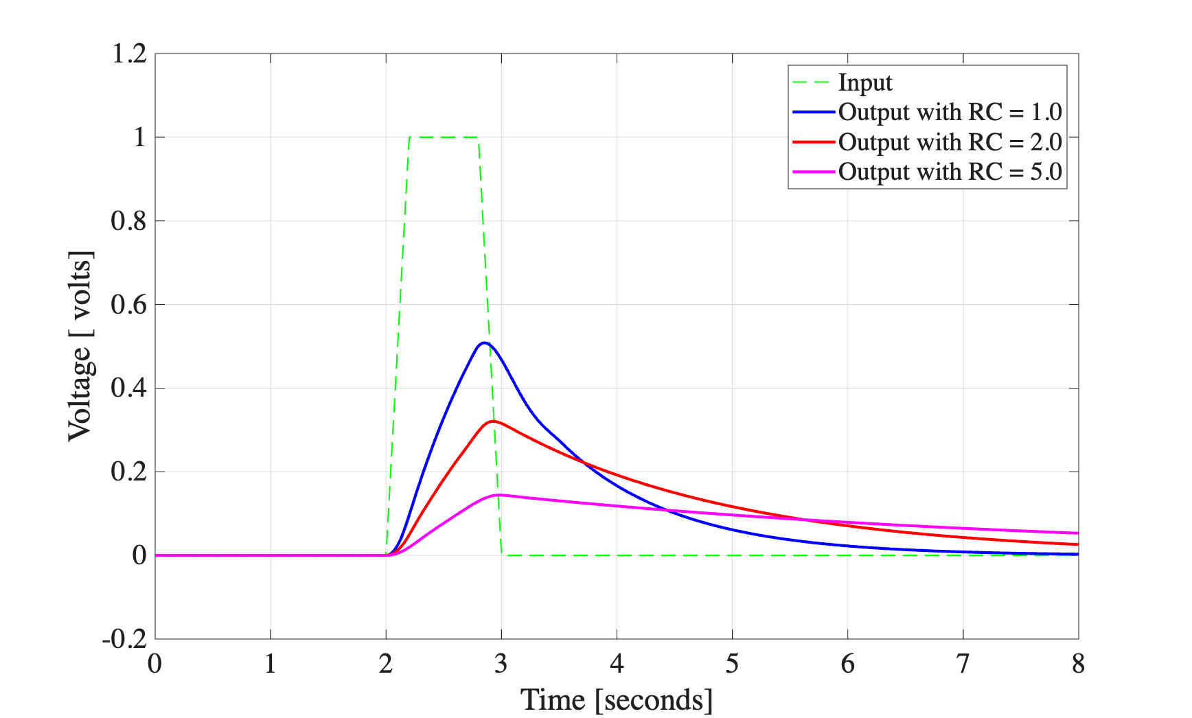

Figure 1: Figure produced by MATLAB script

1.1 The ‘hat response and the time constant’

The values of \(RC\) currently shown in Figure 1 are not fully representative of all the different types of behaviors this system can show. Change the code to show three or four different values of \(RC\) (that may or may not include some of the currently-shown values; it’s up to you) that showcase the different types of behaviors you expect this system to have. Comment on your choices and describe what is happening using the RC circuit. In your comment and description/discussion, you should use the word ‘time constant’.

What to turn in

You do not need to turn in code for this problem. Please turn in your figure and the accompanying discussion.

2 Time-shifted functions

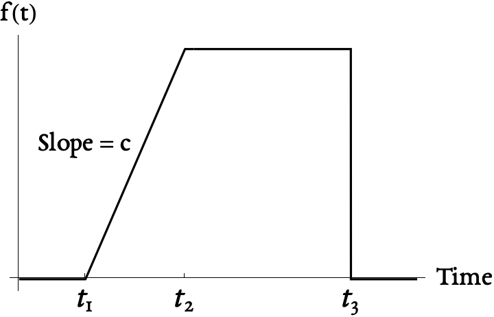
2.1 Obtaining the expression for \(f(t)\)

Write down a mathematical expression, valid for all times \(t\), for the function of time shown below.

2.2 Laplace Transform

Determine an expression for \(F(s)\), the Laplace Transform of the function above. Write it down in two forms: as a rational function, and as a sum of fractions.

2.3 Forced Response: Applying a time-shifted function to a circuit

An RC circuit is set up, as shown below, to which the input voltage is provided according to the following function of time: \[v_{\text{in}}(t) = u_s(t-t_1) \times k \times (t - t_1).\] Here, \(t_1\) is some positive constant and \(u_s\) is the Heaviside step function. Assume that \(RC\), the product of the resistance and capacitance, is some known number.

The capacitor is initially charged, and \(v(0) = v_0\), where \(v_0\) is some positive number.

Determine a mathematical expression for the free response and the forced response of the capacitor voltage in the frequency domain, and in the time domain.

Note

You need four expressions: free response in the time domain, free response in the frequency domain, forced response in the time domain, and forced response in the frequency domain. Your answers will be in terms of \(k\), \(RC\), \(t_1\).

3 Basic Block Diagrams

3.1 One input, one output

Consider the system represented by the following diagram.

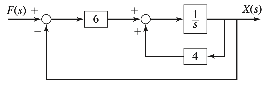
Determine the transfer function \(X(s)/F(s)\).
Draw a simplified version of this block diagram in which there are only two block elements.
Draw a simplified version of this block diagram in which there is only one block element.

3.2 Two inputs, one output

Consider the system represented by the following diagram.

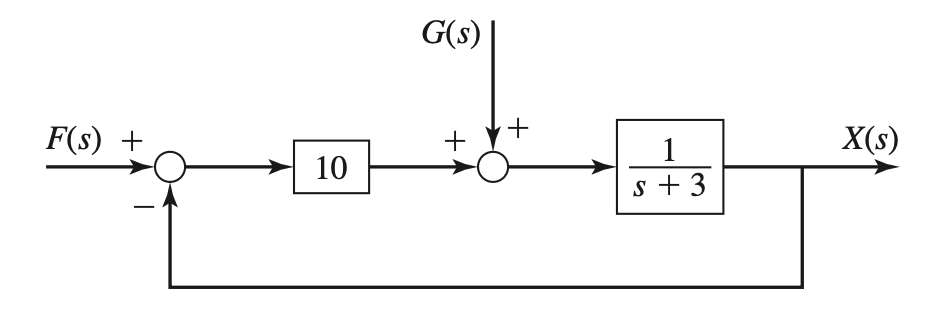
Determine the transfer function \(X(s)/F(s)\)
Determine the transfer function \(X(s)/G(s)\)

3.3 Block Diagram from equations

Draw a block diagram for the following system. The output is \(x(t)\) or \(X(s)\), and the inputs are \(f(t)\) and \(g(t)\) in the time domain, i.e., \(F(s)\) and \(G(s)\) in the frequency domain. Also indicate on your diagram the location of \(Y(s)\).

\[ \begin{aligned} \dot{x} &= y - 5x + g(t) \\ \dot{y} &= 10 f(t) - 30x \end{aligned} \]

Note

The time-dependence of \(x\), \(y\) and their derivatives is assumed in the above equation, and not explicitly written out for neatness.

4 Coupled systems and block diagrams

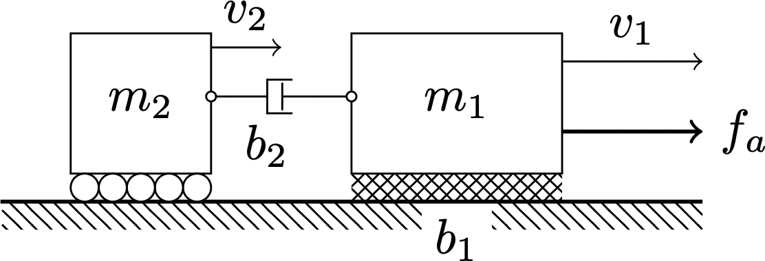
4.1 A Mechanical System

In class, it was shown that the governing equations for the following system of masses and friction elements is

\[ \begin{aligned} m_1 \dot{v}_1 + b_1 v_1 &= f_1 - b_2 v_1 + b_2 v_2 \\ m_2 \dot{v}_2 \phantom{+ b_1 v_1} &= \phantom{f_1 -} b_2 v_1 - b_2 v_2 \end{aligned} \]

The system is shown below.

Figure 3: A mass \(m_1\) is pulled along a friction-full surface by an applied force \(f_a\). A dashpot connects the mass to another mass, \(m_2\), which is supported on the ground by friction-free wheels. The velocities of the two masses, taken positive to the right, are indicated by arrows.

Use the following block diagram to represent the system above. The ‘?’ symbols indicate inputs and outputs.

Warning

This block diagram is not the only way to represent the system in Figure 3. However, you must use the above template to successfully solve this problem.

LaTeX code for block diagram

You may wish to use the LaTeX code for the block diagram.

\documentclass[10pt]{article}
\usepackage[usenames]{color} %used for font color
\usepackage{amssymb} %maths
\usepackage{amsmath} %maths
\usepackage[utf8]{inputenc} %useful to type directly diacritic characters
\usepackage{tikz}
\usetikzlibrary{shapes,arrows,positioning,calc}
\usetikzlibrary{circuits.ee.IEC} 
\tikzset{
block/.style = {draw, fill=white, rectangle, minimum height=3em, minimum width=3em},
tmp/.style  = {coordinate}, 
sum/.style= {draw, fill=white, circle, node distance=1cm},
input/.style = {coordinate},
output/.style= {coordinate},
pinstyle/.style = {pin edge={to-,thin,black}
}
}

\begin{tikzpicture}[thick,auto, node distance=2cm,>=latex']
    \node [input, name=rinput] (rinput) {};
    \node [sum, right of=rinput] (sum1) {};
    \node [block, right of=sum1] (controller) {};
    %\node [block, above of=controller,node distance=1.3cm] (up){$\frac{k_{i\beta}}{s}$};
    %\node [block, below of=controller,node distance=1.3cm] (rate) {$sk_{d\beta}$};
    \node [block, right of=controller,node distance=2cm] (mult) {};
    \node [tmp, below =2cm of mult] (spot) {};
    \node [sum, right of=controller,node distance=4cm] (sum2) {};
    \node [input, above = 1cm of sum2](extra){};  %
    \node [block, right of=sum2,node distance=2cm] (system) {};
    \node [block, below of=system] (feedback) {};
    \node [output, right of=system, node distance=2cm] (output) {};
    \node [output, right of=output] (output2) {};
    \node [tmp, below of=controller] (tmp1){};
    \node [block,right of=tmp1, below = 2.5cm of mult] (feedback1) {};
    %\draw [->] (rinput) -- node{$F(s)$} (sum1);
    \draw [->] (sum1) --node[name=z,anchor=north]{} (controller);
    \draw [->] (controller) -- node[anchor=south]{?} (mult);
    \draw [->] (mult) -- node [coordinate,name=takeoff1] {} (sum2);
    \draw [->] (takeoff1) -- +(0,1) -| (sum1) node[above right] {$+$};
    \draw [->] (sum2) -- node{} (system);
    \draw [->] (system) -- node [name=y] {?}(output2);
    \draw [->] (output) |- (feedback);
    \draw [->] (feedback) -| (sum2) node[below right] {$+$};
    \draw (feedback1) -- (spot);
    \draw [->] (spot) -- (sum2) node[below left=3pt and 7pt] {$+$};
    %\draw [->] (z) |- (rate);
    %\draw [->] (rate) -| (sum2);
    %\draw [->] (z) |- (up);
    %\draw [->] (up) -| (sum2);
    \draw [->] (y) |- (feedback1);
    \draw [->] (feedback1)-| node[pos=0.9] {$+$} (sum1);
    \draw [->] (extra) -- node[above=0.6]{?} (sum2);
    %\draw [->] ($(0,1.5cm)+(extra)$)node[above]{$d_{\beta 2}$} -- (extra);
\end{tikzpicture}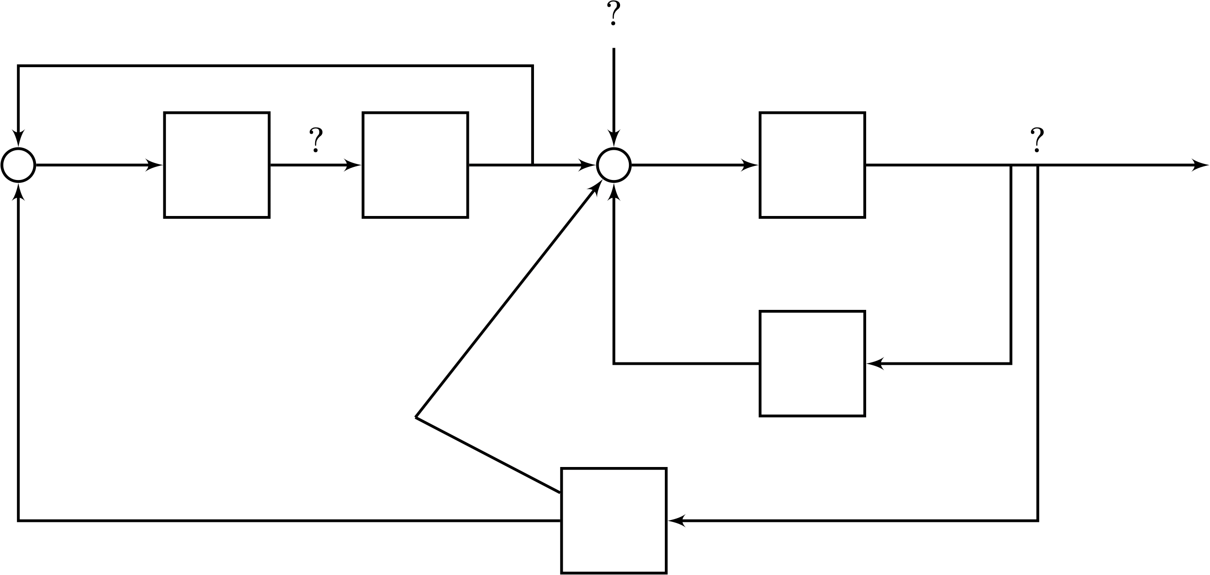

4.2 An Electrical System

Consider the circuit shown below.

Write down a set of coupled differential equations for the voltage across capacitor \(C_1\), \(v_{C_1}\) and the voltage across the capacitor \(C_2\), \(v_{C_2}\).

What the answer should look like

You will have two equations. Each equation should only have one (first-order) derivative. These are \(\dot{v}_{C_1}\) and \(\dot{v}_{C_2}\) respectively. No other derivatives should appear.
You need not put the equations in any special form, but it may be helpful to use the form \((...) \dot{x} + (...) x = ...\)

Draw a block diagram illustrating this system.