Problem Set 7

ENGR 12, Spring 2026.

Due Date	Tue, Mar 17
Turn in link	Gradescope
URL	`emadmasroor.github.io/E12-S26/Homework/HW7`

Points Distribution

Please note that each of the following grade items is a single rubric item. Each rubric item is scored on a four-level scale of 3-2-1-0. You may wish to take this into account when deciding how to allocate your efforts to each problem.

Problem	Part	% Weightage
Problem 1		20
Problem 2	2.1	20
	2.2	20
Problem 3		20
Problem 4		20

1 Classifying second-order systems

1.1 Under-, over- and critically- damped systems

For each of the following systems, determine if you expect the free response to be over-damped, under-damped, or critically damped. Show your work. If a system does not seem to fall into any category, sketch the shape you expect its solution \(x(t)\) to take.

\[\ddot{x} + 4 \dot{x} + 3 x = 0\]
\[\ddot{x} + 3 \dot{x} + 4 x = 0\]
\[2\ddot{x} + \dot{x} + 3 x = 0\]
\[3\ddot{x} + 6\dot{x} + 3 x = 0\]
\[ \ddot{x} + 4\dot{x} -3 x = 0\]
\[2\ddot{x} - 4\dot{x} +3 x = 0\]

Tip

Your sketch does not need to be accurate. Notice that no initial conditions are provided, so we are not looking for a correct graph anyway. Just think about what the solution should qualtiatively look like.

2 Forced (Step) Response of second-order systems

Spring-mass-damper system. Assume that \(x\) has been chosen such that when \(x=0\), there is no push or pull in the spring.

Tip

When a question asks for ‘the unit impulse response’, the ‘unit step response’, or really the ‘something response’, what it’s really asking is this:

Set up the governing differential equation for the system, with the input on the right-hand side. In E12, this will usually look like \(\ddot{x} + \dot{x} + x = f(t)\). Let the input — here, \(f(t)\) — be equal to the ‘something’ the response to which you are asked to find. Then, what is \(x(t)\)?

Note that we usually do not integrate the equation to find the answer, but use other techniques.

2.1 Deriving an expression for the step response

Warning

This question has been clarified to indicate that the spring-mass-damper is underdamped.
A missing factor of \(m\) in Equation 1 was added on Friday March 13

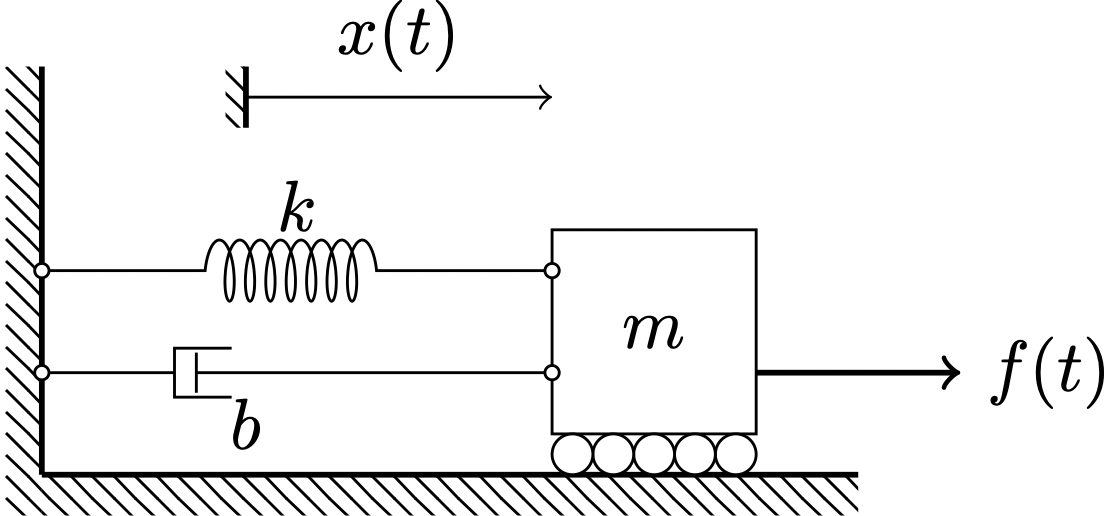
Show that the forced response of an underdamped spring-mass-damper system, such as the one shown above, to a ‘step function force’ equal to \(c\), i.e., the solution of the differential equation \[m \ddot{x} + b \dot{x} + k x = c u_s(t),\] is \[x(t) = \frac{c}{m(r^2+\omega^2)} \left[ 1 - e^{rt} \left( \cos \omega t - \frac{r}{\omega} \sin \omega t \right) \right]. \tag{1}\] Here, \(r\) is the real part of the roots of the characteristic polynomial, and \(\omega\) the imaginary part of the roots of the characteristic polynomial. You should not explicitly leave \(m\), \(b\) and \(k\) in your answer.

Warning

The hand-written part of lecture 14 relevant to this problem had some mistakes; it has been removed from the lecture slides for this reason.

In the process of showing the above, also write down the frequency-domain expression for the forced response, i.e., write down an expression for \(X(s)\) in terms of \(\omega\), \(r\) and \(c\).

Tip

It is possible to solve this problem by using a partial fractions expansion such as \[\frac{1}{s} \frac{1}{m s^2 + b s + k} = \frac{P}{s} + \frac{Q}{s-s_1} + \frac{R}{s-s_2}.\] However, the above strategy is not recommended because it requires using complex \(Q\) and \(R\), which is a huge pain. Instead, it is recommended that you use the following partial fractions expansion: \[\frac{1}{s} \frac{1}{m s^2 + b s + k} = \frac{P}{s} + Q \frac{s-r}{(s-r)^2+\omega^2} + R \frac{\omega}{(s-r)^2+\omega^2}, \tag{2}\] where \(P\), \(Q\) and \(R\) are real constants to be determined (by you).

2.2 Using specific numbers.

For this part, it is OK to just use Equation 1 directly without having to solve any equations.

2.2.1 Expression for \(x(t)\) with numbers

For \(m =1, b = 2, k = 4\) and \(c=2\), write down the expression for \(x(t)\) using numbers and functions. There should be no free parameters here.

2.2.2 Predicting the steady-state response

Recall that the ‘steady-state response’ to an input is how a system behaves in the long run due to the input it receives. For \(m =1, b = 2, k = 4\) and \(c=2\), calculate — without making a plot — the steady-state response, i.e. what value(s) \(x(t)\) takes in the long run.

2.2.3 Making a plot

For \(m =1, b = 2, k = 4\) and \(c=2\), make a plot of \(x(t)\) for the first ten seconds.
Either using your plot or using math, determine the time at which the spring is the farthest from its original position, and write the value of \(t\) and of \(x\) for this instant.

3 The ‘top-hat response’

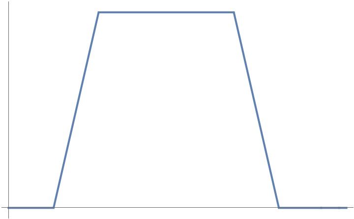
Once again, we would like to examine our system’s behavior in response to a force that is switched on for a period of time and then switched off. We will use a ‘top hat’ function like before, which consists of a ramp up, a constant period, and then a ramp back down to zero.

A spring-mass-damper system is subjected to a force given by the graph shown below.

This function can be specified in MATLAB using

function output = f1(t)
    % Builds a 'hat' from t = 2 to t = 12
    % using ramp functions.
    output = + heaviside(t-2).*5.*(t-2) + ...
             - heaviside(t-4).*5.*(t-4) + ...
             - heaviside(t-10).*5.*(t-10) + ...
             + heaviside(t-12).*5.*(t-12);
end

The differential equation can be implemented in MATLAB using

function dydt = rhs1(t,y,m)
% Define the right-hand side function of differential equation. It takes as
% input the value of m, which is a parameter we will change, in addition to
% the usual "t" and "y", where "y" is the state variable.
    b = 2; k = 4;

    x = y(1);
    xdot = y(2);

    dy1dt = xdot;
    dy2dt = (-b*xdot - k*x + f1(t))/m;

    dydt= [dy1dt;dy2dt];
end

Use the following starter code to investigate three values of \(m\) that show qualitatively different kinds of behaviorss. Describe how the behaviors you see are qualitatively different from each other.

% Define a time domain with lots of values
N     = 1000;
tvals = linspace(0,40,N);

% Call ode45 with initial conditions of zero using various values for m.
[t1,x1] = ode45(@(t,x) rhs1(t,x,1), tvals, [0;0]);

% Plot response 
clf;
yyaxis right;
plot(tvals,f1(tvals),'--',"LineWidth",1,'Color',"black");  hold on;
ylabel("Applied force f(t)")
yyaxis left;
plot(tvals,x1(:,1),'-',"LineWidth",2,"Color","blue"); hold on;
ylabel("Response x(t)")

% Make it pretty
set(gca,"FontSize",14);
pbaspect([3,1,1]);
xlabel("Time");

What to turn in

Do not turn in .m files. It is sufficient to provide only your MATLAB figure and an accompanying explanation, which should be a few sentences long (up to one paragraph).

4 RLC Circuits

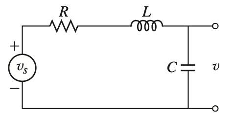
For the RLC circuit shown, it is known that the governing equation for the voltage across the capacitor is \[LC \ddot{v} + RC \dot{v} + v = v_s.\] When there is no input voltage and just a free response, what is the

Undamped natural frequency,
Damping ratio, and
Damped natural frequency

for the system? Give your answers in terms of \(R\), \(L\) and \(C\).