Lecture 5
E12 Linear Physical Systems Analysis
What do we do when \(f(t)\) is more complicated?
For first-order systems, \[\dot{x} + a x = f(t).\]
If integrating \(f(t)\) is too difficult, we can …
- give up, and integrate using
ode45orsolve_ivp - or … ?
- give up, and integrate using
Numerical solutions mask deeper insight and do not give a full picture of the solution.
Need a new way of looking at problems …
The Frequency Domain
Laplace Transform
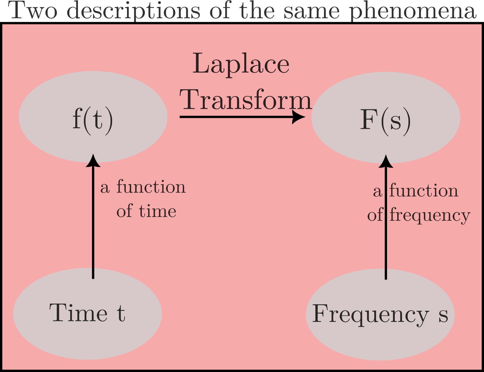
- The Laplace Transform of a function transforms the function from the time domain to the frequency domain.
- What is the domain of a function?
- “The set of inputs accepted by the function”
\[\boxed{f(t) \rightarrow F(s)}\]
- Lowercase letters: time domain functions
- Uppercase letters: frequency domain functions
- \(s\) is complex, actually (but don’t worry about it for now!)
Time domain and Frequency Domain
Defining the Laplace Transform
- The Laplace Transform of a function \(x(t)\) is defined as the following function of \(s\): \[\lim_{T \rightarrow \infty} \int_0^{T} x(t)e^{-st} dt \tag{1}\]
- This is a function of \(s\), not a function of \(t\).
- We give the expression in Equation 1 the name \(X(s)\) \[X(s) = \boxed{\lim_{T \rightarrow \infty} \int_0^{T} x(t)e^{-st} dt} = \int_0^{\infty} x(t)e^{-st} dt\] \[x(t) \rightarrow \text{Laplace Transform} \rightarrow X(s) \] \[x(t) \rightarrow \mathcal{L}[\cdot] \rightarrow X(s)\] \[\boxed{\mathcal{L}[x(t)] = X(s)}\]
Derive the Laplace Transform for a simple function \(x(t) = 3\)
If \(x(t) = 3\), a constant, what is \(\mathcal{L}[x(t)]\), i.e., what is \(X(s)\) ?
\[ \boxed{ \begin{aligned} \mathcal{L}[3] &= \int_0^{\infty} 3 e^{-st} dt \\ &= 3 \times \frac{1}{-s} \left. e^{-st} \right|_0^{\infty} \\ &= \frac{3}{-s} \left( e^{-\infty} - e^0 \right) \\ &= \frac{3}{s} \end{aligned} } \]
Derive the Laplace Transform for a simple function \(x(t) = e^{-at}\)
If \(x(t) = e^{-at}\), what is \(\mathcal{L}[x(t)]\), i.e., what is \(X(s)\) ?
\[ \boxed{ \begin{aligned} \mathcal{L}[e^{-at}] &= \lim_{T \rightarrow \infty}\int_0^T e^{-at} e^{-st} dt \\ &= \lim_{T \rightarrow \infty} \int_0^T e^{-(s+a)t} dt \\ &= \lim_{T \rightarrow \infty} \left[ \frac{-1}{s+a} e^{-(s+a)t} \right]_{t=0}^{t=T} \\ &= \frac{1}{s+a} \end{aligned} } \]
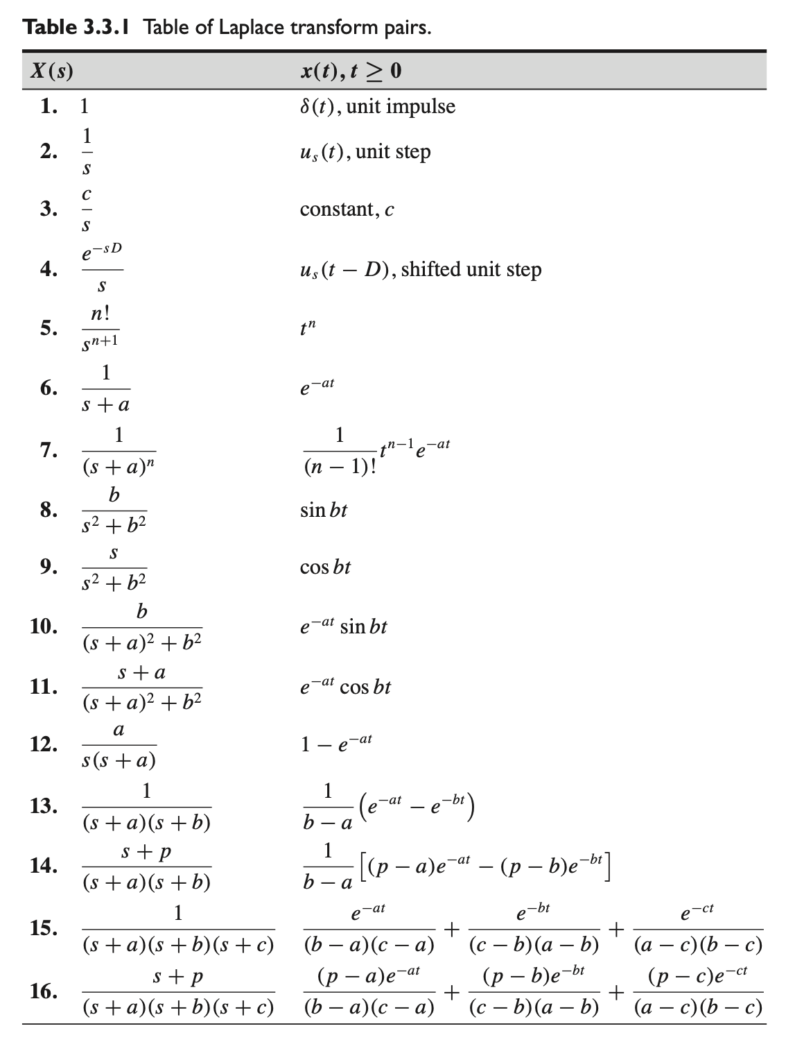
Table of Laplace Transforms
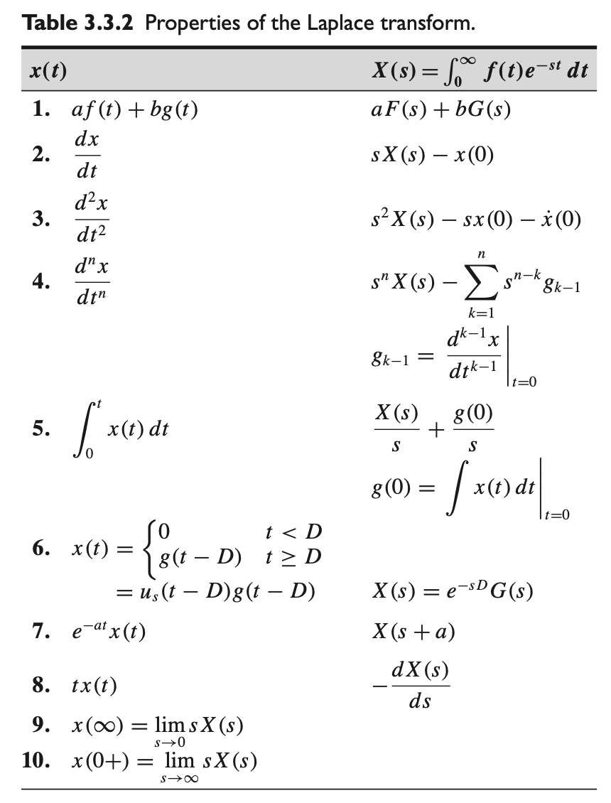
Properties of Laplace Transforms
The Inverse Laplace Transform
- Time domain → Frequency domain: Laplace Transform
- Time domain ← Frequency domain: ??
- Inverse Laplace Transform
\[\boxed{F(s)\rightarrow f(t)}\]
- We will not learn how to calculate the inverse transform directly. Instead:
- Pattern matching!
Identifying the inverse Laplace transform
- We have already learned that
\[ \begin{aligned} \mathcal{L}[3] &= \frac{3}{s} \\ \mathcal{L}[e^{-at}] &= \frac{1}{s+a} \end{aligned} \]
- So the inverse Laplace transforms are
\[ \begin{aligned} \mathcal{L^{-1}}\left[\frac{3}{s}\right] &= 3 \\ \mathcal{L^{-1}}\left[\frac{1}{s+a}\right] &= e^{-at} \end{aligned} \]
Linearity Property of the Laplace Transform
\[ \boxed{ \begin{aligned} \mathcal{L}\left[ a f(t) + b g(t) \right] &= a \mathcal{L}\left[ f(t) \right] + b \mathcal{L} \left[ g(t) \right] \\ &= a F(s) + b G(s) \end{aligned} } \]
- The Laplace Transform of the sum of two functions equals the sum of the Laplace Transform of those two functions.
- The Laplace Transform of \(k \times\) a function equals \(k \times\) the Laplace Transform of that function.
- The inverse Laplace Transform is similarly linear: \[ \boxed{ \begin{aligned} \mathcal{L^{-1}}\left[ a F(s) + b G(s) \right] &= a \mathcal{L^{-1}}\left[ F(s) \right] + b \mathcal{L^{-1}} \left[ G(s) \right] \\ &= a f(t) + b g(t) \end{aligned} } \]
Using the Linearity Property to find \(\mathcal{L}[x(t)]\)
Given \[x(t) = 6 + 4 e^{-3t},\] find \(\mathcal{L}[ x(t)]\)
a.k.a. \(X(s)\)
a.k.a. “Laplace transform of \(x(t)\)”.
\[ \boxed{ \begin{aligned} \mathcal{L}\left[ a f(t) + b g(t) \right] &= a \mathcal{L}\left[ f(t) \right] + b \mathcal{L} \left[ g(t) \right] \\ &= a F(s) + b G(s) \end{aligned} } \]
\[ \boxed{ \begin{aligned} \mathcal{L}\left[ 6+4e^{-3t} \right] &= \mathcal{L}[6] + \mathcal{L}\left[ 4e^{-3t}\right] \\ &= 2 \cdot \mathcal{L}[3] + 4 \cdot \mathcal{L}\left[ e^{-3t}\right] \\ &= 2 \cdot \underbrace{\frac{3}{s}}_{\mathcal{L}[3]} + 4 \cdot \underbrace{\frac{1}{s+3}}_{\mathcal{L}\left[ e^{-3t}\right]} = \frac{6(s+3) + 4s}{s(s+3)} \end{aligned} } \]
The Derivative Property of Laplace Transforms
- Even without knowing exactly what \(x(t)\) is, we can transform first derivatives: \[\mathcal{L} \left[ \frac{dx}{dt} \right] = s \mathcal{L} \left[ x(t) \right] - x(0)\]
- and second derivatives: \[\mathcal{L} \left[ \frac{d^2x}{dt^2} \right] = s^2 \mathcal{L} \left[ x(t) \right] - s x(0) - \dot{x}(0)\]
Derivation (without much nuance re: limits): \[ \boxed{ \begin{aligned} \mathcal{L}\left[ \frac{dx}{dt}\right] = \int_0^{\infty} \frac{dx}{dt} e^{-st} dt &= \left. x(t) e^{-st} \right|_0^{\infty} + s \underbrace{\int_0^{\infty} x(t) e^{-st} dt}_{\mathcal{L}[x(t)]} \\ &= \left(x(\infty) e^{-\infty} - x(0) e^{0} \right) + s X(s) \\ &= sX(s)-x(0) \end{aligned} } \] and repeated application of the above procedure gives us \(\displaystyle \mathcal{L} \left[ \frac{d^n x}{dt^n} \right]\)
Laplace Transform to solve 1st-order system
- Consider the general first-order system \[ \dot{x} + a x = f(t)\]
- Apply \(\mathcal{L}[\cdot]\) to both sides
\[s X(s) - x(0) + a X(s) = F(s)\]
- Collect \(X(s)\) terms together and solve for \(X\):
\[ \begin{aligned} X(s) \cdot (s+a) &= F(s) + x(0) \\ X(s) &=\frac{F(s)}{s+a} + \frac{x(0)}{s+a} \end{aligned} \]
- Apply \(\mathcal{L}^{-1}\): \(\boxed{\displaystyle x(t) = \mathcal{L}^{-1} \left[ \frac{F(s)}{s+a} + \frac{x(0)}{s+a}\right]}\)
A familiar problem but with Laplace
\[RC \dot{v} + v = v_s \text{(const.)}, \quad v(0) = 0\]
Using the Laplace Transform to solve IVPs
Solve \[\dot{x} + 2x = 6+4 e^{-3t}, \quad x(0) = 0\] using Laplace Transforms:
- first find \(X(s)\)
- then use \(\mathcal{L}^{-1}\) to find \(x(t)\)
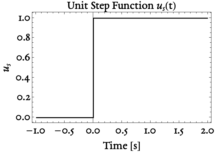
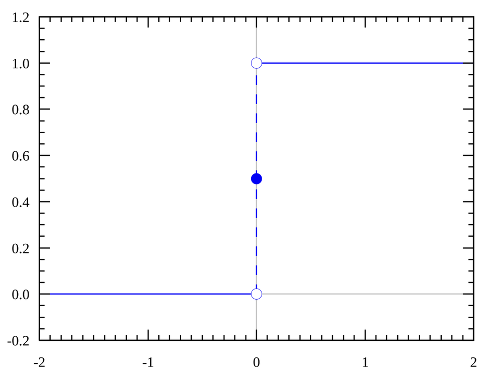
Two new functions: The Heaviside Step function
a.k.a. the “unit step function”:
\[u_s(t) = \begin{cases} 0 & {t < 0} \\ 1 & {t>0} \end{cases}\]
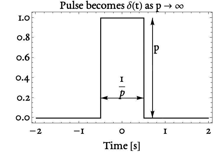
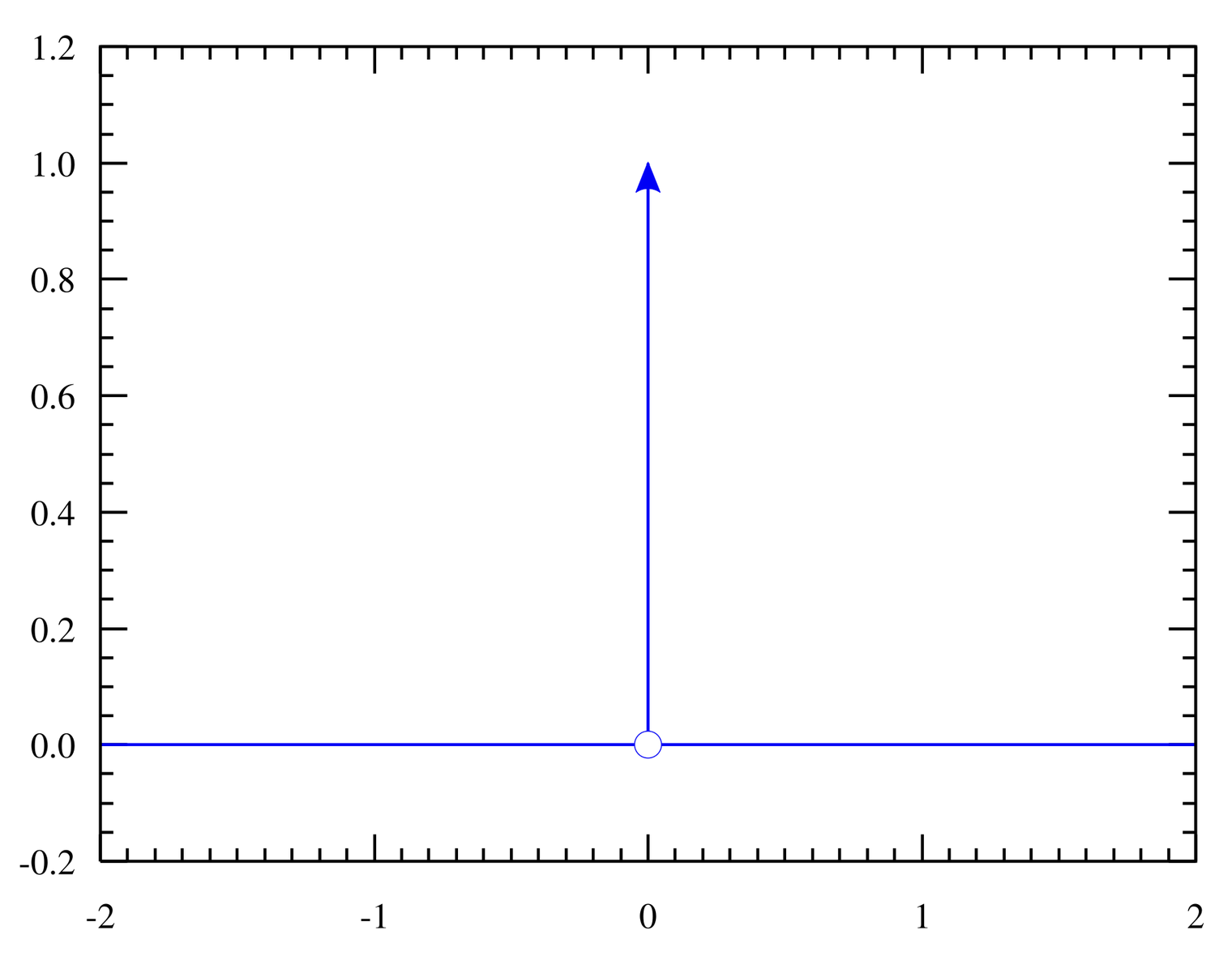
Two new functions: The Dirac Delta function
a.k.a. the “impulse”:
\[\delta(t) = \begin{cases} 0 & {t \neq 0} \\ \infty & {t = 0} \end{cases}\]
such that \(\displaystyle \int_{-\infty}^{+\infty} \delta(t) = 1\)
The Step function and the Impulse Function
\[\boxed{\frac{d}{dt} \left( u_s(t) \right) = \delta(t)}\]
Rational Functions & Partial Fractions Expansion
A rational function is any function that can be expressed as a fraction in which the numerator and denominator are both polynomials.
Express the following rational function as a sum of fractions:
\[\frac{10s+18}{s(s+3)^2} = \frac{A}{s} + \frac{B}{s+3} + \frac{C}{(s+3)^2}\]
Partial Fractions Expansion
For a given rational function \[\frac{p(s)}{q(s)} \] where \(p(s)\) is of lower or equal degree than \(q(s)\),
write the function as \[\frac{p(s)}{q(s)} = \frac{(s-p_1)(s-p_2)(...)(s-p_m)}{(s-q_1)(s-q_2)(s-q_3)... (s-q_n)}\]
where \(p_i\) is the \(i\) ’th root of \(p(s)\) and \(q_i\) is the \(i\) ’th root of \(q(s)\).
It is possible to find constants \(A\), \(B\), \(C\), … such that \[\frac{p(s)}{q(s)} = \frac{A}{s-q_1} + \frac{B}{s-q_2} + \frac{C}{s-q_3} + ...\]
If any roots are repeated, the corresponding term appears once for each time the root is repeated.
For example, if \(q(s) = s (s+3)^2,\) then the partial fraction expansion will be \[\frac{A}{s} + \frac{B}{s+3} + \frac{C}{(s+3)^2}\]
For example, if \(q(s) = s^2 (s+3),\) then the partial fraction expansion will be \[\frac{A}{s} + \frac{B}{s^2} + \frac{C}{s+3} \]