Problem Set 12 Solutions

ENGR 12, Spring 2026.

Solutions

1 Moving a system of two masses

1.1 Derive the state-space equations

Derive the state-space equations for the above system, considering \(f_a(t)\) to be the sole input and \(x_2-x_1\) to be the sole output. Let \(m_1=m_2=m\). Use the state variables

\(\dot{x}_1\)
\(\dot{x}_2\)
\(x_2-x_1\)

Solutions

Using the following FBD diagram,

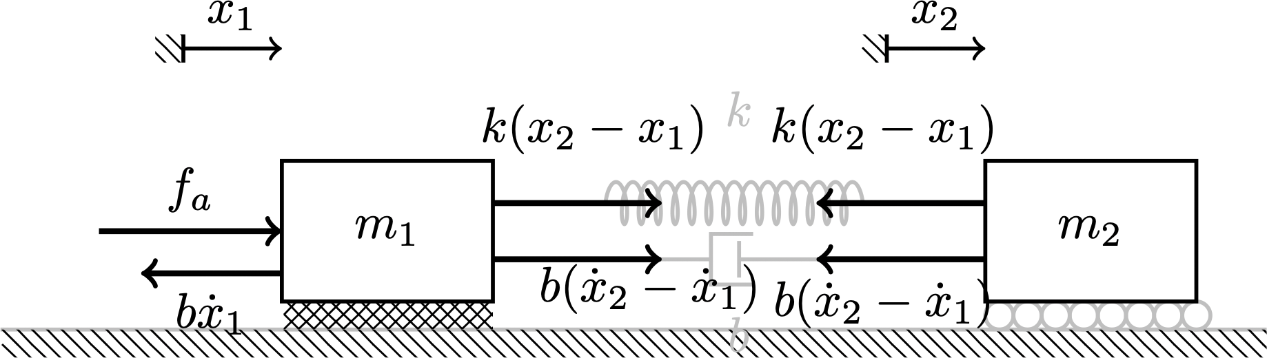
we can write Newton’s second law for the two masses seaprately.

For mass 1, we have \[m\ddot{x}_1 = k(x_2-x_1) + b(\dot{x}_2-\dot{x}_1) + f_a - b \dot{x}_1\]
For mass 2, we have \[m\ddot{x}_2 = -k(x_2-x_1) - b(\dot{x}_2-\dot{x}_1)\]

The state-space equations are \[ \begin{aligned} \frac{d}{dt} \begin{bmatrix} \dot{x}_1 \\ \dot{x}_2 \\ z \end{bmatrix} &= \begin{bmatrix} \displaystyle -\frac{2b}{m} & \displaystyle \frac{b}{m} & \displaystyle \frac{k}{m} \\ \displaystyle \frac{b}{m} & \displaystyle -\frac{b}{m} & \displaystyle -\frac{k}{m} \\ -1 & 1 & 0 \end{bmatrix} \cdot \begin{bmatrix} \dot{x}_1 \\ \dot{x}_2 \\ z \end{bmatrix} + \begin{bmatrix} 1/m \\ 0 \\ 0 \end{bmatrix} \cdot \begin{bmatrix} f_a \end{bmatrix} \\ {\boldsymbol{y}} &= \boldsymbol{C} \boldsymbol{x} + \boldsymbol{D} \boldsymbol{u} \end{aligned} \]

where \(\boldsymbol{y}\) is the output vector. If the only output is the third state variable, \(z = x_2-x_1\), the matrix \(C = [0,0,1]\) and the matrix \(D = [0]\).

1.2 Explore in MATLAB

Note

For the entirety of Section 1.2, the physical system is identical to Figure 2, but the outputs we are interested in are different from the output in Section 1.1. We are now interested in the following two outputs:

\(\dot{x}_1\)
\(\dot{x}_2\)

Use the following parameter values: \(b=5\), \(m=1\) and \(k=3\).

Hint

Consider which of the matrices A, B, C and D need to change before you can use MATLAB. Also check out this slide to make sure the dimensions of your matrices are correct.

1.2.1 Transfer Functions using MATLAB

Use the ss and tf functions to determine the transfer function between the input \(f_a\) and the two outputs:

\(\dot{x}_1\)
\(\dot{x}_2\)

Give your answer in the form of a rational function of \(s\), the frequency variable.

Solutions

The following MATLAB code was used.

b = 5;
m = 1;
k = 3;

A = [-2*b/m, b/m, k/m;
     b/m, -b/m, -k/m;
     -1, 1, 0];

B = [1/m;
     0;
     0];

% Output = the first and second state variables
C = [1,0,0;
     0,1,0];

D = [0;
     0];

sys1 = ss(A, B, C, D);
tfsys1 = tf(sys1)

This gave the following output:

  From input to output...
            s^2 + 5 s + 3
   1:  ------------------------
       s^3 + 15 s^2 + 31 s + 15
 
               5 s + 3
   2:  ------------------------
       s^3 + 15 s^2 + 31 s + 15

i.e., the desired transfer functions are:

From input \(f_a\) to output \(\dot{x}_1\): \[ \frac{s^2+5s+3}{s^3+15s^2+31s+15}\]
From input \(f_a\) to output \(\dot{x}_2\): \[ \frac{5s+3}{s^3 + 15 s^2 + 31s + 15}\]

1.2.2 Poles in MATLAB

You will notice that the transfer functions you have found in Section 1.2.1 have third-degree polynomials in \(s\) in their denominator. This tells us that the system is third order, and there should be three poles.

Tip

Recall that a pole is a value of \(s\) that would make the transfer function undefined. A pole of a transfer function is also a root of the denominator polynomial of that transfer function.

Determine the numerical value of the three poles of this system. To do this, you may either use MATLAB’s pole function, or use a computer algebra program such as WolframAlpha to find the roots of the cubic polynomial in the denominator.

Give your answer as a set of three (possibly complex) numbers.

Solutions

Following on from the last part’s MATLAB code, we can use

>> pole(tfsys1)

ans =

  -12.6416
   -1.6307
   -0.7276

So the three poles are \(-12.6, -1.63, -0.73\).

1.2.3 Zeros in MATLAB

A transfer function has zeros in addition to poles.

Tip

Recall that a zero of a transfer function is a value of \(s\) that would make the transfer function equal to zero. A zero of a transfer function is also a root of the numerator polynomial of that transfer function.

Find the zeros of each of the transfer functions that you found in Section 1.2.1. You can either do this mathematically or you can use the zero function of MATLAB.

Note

The MATLAB function zero only works for ‘single-input, single-output’ systems, not for multiple-input or multiple-output systems. However, it is still possible to use zero here by extracting two separate transfer functions out of the output of tf from your answer to Section 1.2.1.

Solutions

Following on from the last part’s MATLAB code, we can use

>> zero(tfsys1(1))

ans =

   -4.3028
   -0.6972

>> zero(tfsys1(2))

ans =

   -0.6000

So the zeros are:

For the output \(\dot{x}_1\): \(s = -4.30, \quad s= -0.70\)
For the output \(\dot{x}_2\): \(s = -3/5\)

1.2.4 Impulse Response

We would like to examine the response of this system to an impulse input where \(f_a(t)\) takes the form of a Dirac Delta function. Use MATLAB’s impulse function to produce a time-domain plot of how \(\dot{x}_1\) and \(\dot{x}_2\) respond to such an input. It is okay to directly reproduce MATLAB’s plots without any modification.

Also write a brief description of what this represents physically.

Solutions

The impulse response is as follows.

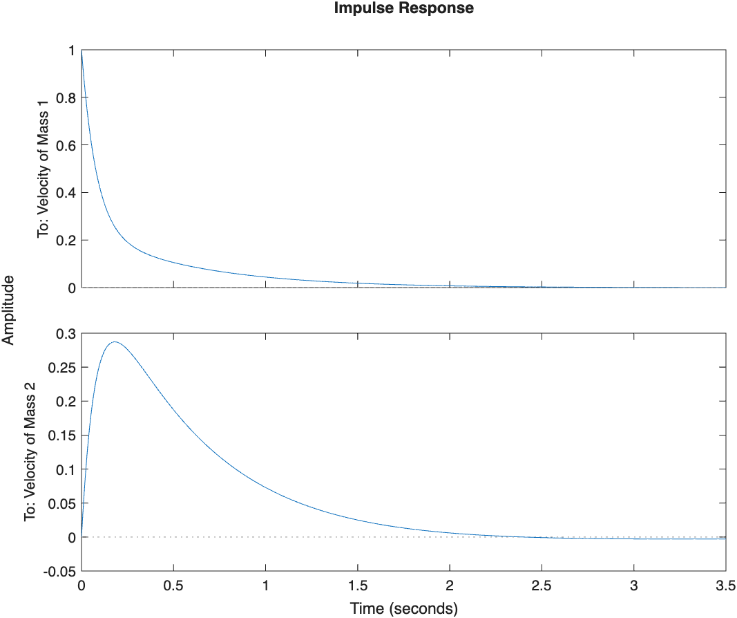
It was determined using the code

sys1.OutputName= {'Velocity of Mass 1','Velocity of Mass 2'};
impulse(sys1)

Physically, this suggests that if mass 1 is struck with an impulse, it will start at a large velocity and slow down until it comes to a rest. Meanwhile mass 2 will respond by slowly picking up speed until a certain amount of time has passed, after which it will start slowing down and gradually come to a stop as well.

1.3 Repeat with a smaller \(b\) value

Repeat Section 1.2.1, Section 1.2.2, Section 1.2.3, and Section 1.2.4 for the following system parameters, and briefly comment on the differences you observe (one to two sentences).

\(m=1, k = 3, b = 0.2\).

Solutions

Transfer functions

  From input to output...
             s^2 + 0.2 s + 3
   1:  ----------------------------
       s^3 + 0.6 s^2 + 6.04 s + 0.6
 
                0.2 s + 3
   2:  ----------------------------
       s^3 + 0.6 s^2 + 6.04 s + 0.6

For \(\dot{x}_1\): \[\frac{s^2+0.2s+3}{s^3+0.6s^2+6.04s+0.6} \tag{1}\]
For \(\dot{x}_2\): \[\frac{0.2s+3}{s^3+0.6s^2+6.04s+0.6} \tag{2}\]

Poles

The poles of this system are located at

  -0.2499 + 2.4346i
  -0.2499 - 2.4346i
  -0.1002 + 0.0000i

Zeros

The zeros of Equation 1 are located at

  -0.1000 + 1.7292i
  -0.1000 - 1.7292i

Tehre is only one zero of Equation 2 and it is located at

-15.000

Impulse Response

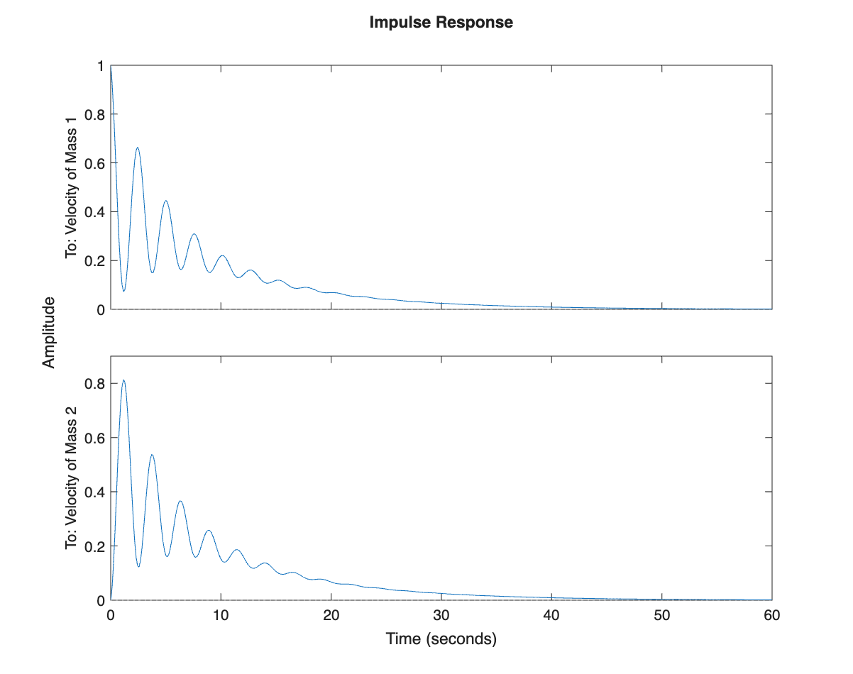
Comment

We notice that the system now has complex poles, and there is oscillation consistent with ‘underdamping’. This suggests that the earlier value of \(b=5\) was overdamped, whereas \(b=0.2\) is underdamped.

2 The shape of matrices in state-space equations

Write out a sample set of matrices and vectors (the entries are irrelevant; the size and shape of the matrices are what you should pay attention to) for the state-space equations when a linear physical system has:

Three state variables, 3 outputs, and 2 inputs.
Two state variables, 1 input, and 3 outputs.
Two state variables, 1 output, and 3 inputs.
Four state variables, 2 inputs, and 4 outputs that are identical to the state variables. (for this one, your matrix \(C\) and \(D\) must have the numerically correct entries)

For each part, write down:

The matrices A, B, C and D with the correct shape and dummy entries.
The vectors \(\boldsymbol{u}\), \(\boldsymbol{x}\) and \(\boldsymbol{y}\) with entries labeled with \(u_1\), \(u_2\), … \(x_1\), \(x_2\), …, and \(y_1\), \(y_2\), ….
The state-space equation in full form.

Solutions

2.1 Three state variables, 3 outputs, 2 inputs

The matrices are: \[ A = \begin{bmatrix} A_{11} & A_{12} & A_{13} \\ A_{21} & A_{22} & A_{23} \\ A_{31} & A_{32} & A_{33} \end{bmatrix}, \quad B = \begin{bmatrix} B_{11} & B_{12} \\ B_{21} & B_{22} \\ B_{31} & B_{32} \end{bmatrix}, \quad C = \begin{bmatrix} C_{11} & C_{12} & C_{13} \\ C_{21} & C_{22} & C_{23} \\ C_{31} & C_{32} & C_{33} \end{bmatrix}, \quad D = \begin{bmatrix} D_{11} & D_{12} \\ D_{21} & D_{22} \\ D_{31} & D_{32} \end{bmatrix} \]
The vectors are: \[ \boldsymbol{x} = \begin{bmatrix} x_1 \\ x_2 \\ x_3 \end{bmatrix}, \quad \boldsymbol{u} = \begin{bmatrix} u_1 \\ u_2 \end{bmatrix}, \quad \boldsymbol{y} = \begin{bmatrix} y_1 \\ y_2 \\ y_3 \end{bmatrix} \]
The equations can be written as: \[ \begin{aligned} \frac{d}{dt} \begin{bmatrix} x_1 \\ x_2 \\ x_3 \end{bmatrix} &= \begin{bmatrix} A_{11} & A_{12} & A_{13} \\ A_{21} & A_{22} & A_{23} \\ A_{31} & A_{32} & A_{33} \end{bmatrix} \cdot \begin{bmatrix} x_1 \\ x_2 \\ x_3 \end{bmatrix} + \begin{bmatrix} B_{11} & B_{12} \\ B_{21} & B_{22} \\ B_{31} & B_{32} \end{bmatrix} \cdot \begin{bmatrix} u_1 \\ u_2 \end{bmatrix} \\ \begin{bmatrix} y_1 \\ y_2 \\ y_3 \end{bmatrix} &= \begin{bmatrix} C_{11} & C_{12} & C_{13} \\ C_{21} & C_{22} & C_{23} \\ C_{31} & C_{32} & C_{33} \end{bmatrix} \cdot \begin{bmatrix} x_1 \\ x_2 \\ x_3 \end{bmatrix} + \begin{bmatrix} D_{11} & D_{12} \\ D_{21} & D_{22} \\ D_{31} & D_{32} \end{bmatrix} \cdot \begin{bmatrix} u_1 \\ u_2 \end{bmatrix} \end{aligned} \]

2.2 Two state variables, 1 input and 3 outputs

The matrices are: \[ A = \begin{bmatrix} A_{11} & A_{12}\\ A_{21} & A_{22} \end{bmatrix}, \quad B = \begin{bmatrix} B_{11} \\ B_{21} \end{bmatrix}, \quad C = \begin{bmatrix} C_{11} & C_{12} \\ C_{21} & C_{22} \\ C_{31} & C_{32} \end{bmatrix}, \quad D = \begin{bmatrix} D_{11} \\ D_{21} \\ D_{31} \end{bmatrix} \]
The vectors are: \[ \boldsymbol{x} = \begin{bmatrix} x_1 \\ x_2 \end{bmatrix}, \quad \boldsymbol{u} = \begin{bmatrix} u_1 \end{bmatrix}, \quad \boldsymbol{y} = \begin{bmatrix} y_1 \\ y_2 \\ y_3 \end{bmatrix} \]
The equations can be written as: \[ \begin{aligned} \frac{d}{dt} \begin{bmatrix} x_1 \\ x_2 \end{bmatrix} &= \begin{bmatrix} A_{11} & A_{12}\\ A_{21} & A_{22} \end{bmatrix} \cdot \begin{bmatrix} x_1 \\ x_2 \end{bmatrix} + \begin{bmatrix} B_{11} \\ B_{21} \end{bmatrix} \cdot \begin{bmatrix} u_1 \end{bmatrix} \\ \begin{bmatrix} y_1 \\ y_2 \\ y_3 \end{bmatrix} &= \begin{bmatrix} C_{11} & C_{12} \\ C_{21} & C_{22} \\ C_{31} & C_{32} \end{bmatrix} \cdot \begin{bmatrix} x_1 \\ x_2 \end{bmatrix} + \begin{bmatrix} D_{11} \\ D_{21} \\ D_{31} \end{bmatrix} \cdot \begin{bmatrix} u_1 \end{bmatrix} \end{aligned} \]

2.3 Two state variables, 1 output and 3 inputs

The matrices are: \[ A = \begin{bmatrix} A_{11} & A_{12}\\ A_{21} & A_{22} \end{bmatrix}, \quad B = \begin{bmatrix} B_{11} & B_{12} & B_{13} \\ B_{21} & B_{22} & B_{23} \end{bmatrix}, \quad C = \begin{bmatrix} C_{11} & C_{12} \end{bmatrix}, \quad D = \begin{bmatrix} D_{11} & D_{12} & D_{13} \end{bmatrix} \]
The vectors are: \[ \boldsymbol{x} = \begin{bmatrix} x_1 \\ x_2 \end{bmatrix}, \quad \boldsymbol{u} = \begin{bmatrix} u_1 \\ u_2 \\ u_3 \end{bmatrix}, \quad \boldsymbol{y} = \begin{bmatrix} y_1 \end{bmatrix} \]
The equations can be written as: \[ \begin{aligned} \frac{d}{dt} \begin{bmatrix} x_1 \\ x_2 \end{bmatrix} &= \begin{bmatrix} A_{11} & A_{12}\\ A_{21} & A_{22} \end{bmatrix} \cdot \begin{bmatrix} x_1 \\ x_2 \end{bmatrix} + \begin{bmatrix} B_{11} \\ B_{21} \end{bmatrix} \cdot \begin{bmatrix} u_1 \end{bmatrix} \\ \begin{bmatrix} y_1 \end{bmatrix} &= \begin{bmatrix} C_{11} & C_{12} \end{bmatrix} \cdot \begin{bmatrix} x_1 \\ x_2 \end{bmatrix} + \begin{bmatrix} D_{11} & D_{12} & D_{13} \end{bmatrix} \cdot \begin{bmatrix} u_1 \\ u_2 \\ u_3 \end{bmatrix} \end{aligned} \]

2.4 Four state variables, 2 inputs and 4 outputs

Where the outptus are just the state variables.

The matrices are: \[ A = \begin{bmatrix} A_{11} & A_{12} & A_{13} & A_{14}\\ A_{21} & A_{22} & A_{23} & A_{24}\\ A_{31} & A_{32} & A_{33} & A_{34}\\ A_{41} & A_{42} & A_{43} & A_{44} \end{bmatrix}, \quad B = \begin{bmatrix} B_{11} & B_{12} \\ B_{21} & B_{22} \\ B_{31} & B_{32} \\ B_{41} & B_{42} \end{bmatrix}, \quad C = \begin{bmatrix} C_{11} & C_{12} & C_{13} & C_{14}\\ C_{21} & C_{22} & C_{23} & C_{24}\\ C_{31} & C_{32} & C_{33} & C_{34}\\ C_{41} & C_{42} & C_{43} & C_{44} \end{bmatrix}, \quad D = \begin{bmatrix} D_{11} & D_{12} \\ D_{21} & D_{22} \\ D_{31} & D_{32} \\ D_{41} & D_{42} \end{bmatrix} \] Where we know that \[C = \begin{bmatrix} 1 & 0 & 0 & 0\\ 0 & 1 & 0 & 0\\ 0 & 0 & 1 & 0\\ 0 & 0 & 0 & 1 \end{bmatrix}, \quad D = \begin{bmatrix} 0 & 0 \\ 0 & 0 \\ 0 & 0 \\ 0 & 0 \end{bmatrix}\]
The vectors are: \[ \boldsymbol{x} = \begin{bmatrix} x_1 \\ x_2 \\ x_3 \\ x_4 \end{bmatrix}, \quad \boldsymbol{u} = \begin{bmatrix} u_1 \\ u_2 \end{bmatrix}, \quad \boldsymbol{y} = \begin{bmatrix} y_1 \\ y_2 \\ y_3 \\ y_4 \end{bmatrix} \]
The equations can be written as: \[ \begin{aligned} \frac{d}{dt} \begin{bmatrix} x_1 \\ x_2 \end{bmatrix} &= \begin{bmatrix} A_{11} & A_{12} & A_{13} & A_{14}\\ A_{21} & A_{22} & A_{23} & A_{24}\\ A_{31} & A_{32} & A_{33} & A_{34}\\ A_{41} & A_{42} & A_{43} & A_{44} \end{bmatrix} \cdot \begin{bmatrix} x_1 \\ x_2 \\ x_3 \\ x_4 \end{bmatrix} + \begin{bmatrix} B_{11} & B_{12} \\ B_{21} & B_{22} \\ B_{31} & B_{32} \\ B_{41} & B_{42} \end{bmatrix} \cdot \begin{bmatrix} u_1 \\ u_2 \end{bmatrix} \\ \begin{bmatrix} y_1 \\ y_2 \\ y_3 \\ y_4 \end{bmatrix} &= \begin{bmatrix} 1 & 0 & 0 & 0\\ 0 & 1 & 0 & 0\\ 0 & 0 & 1 & 0\\ 0 & 0 & 0 & 1 \end{bmatrix} \cdot \begin{bmatrix} x_1 \\ x_2 \\ x_3 \\ x_4 \end{bmatrix} + \begin{bmatrix} 0 & 0 \\ 0 & 0 \\ 0 & 0 \\ 0 & 0 \end{bmatrix} \cdot \begin{bmatrix} u_1 \\ u_2 \end{bmatrix} \end{aligned} \]

3 A vibration isolation system

Consider the following system, which is a simplified representation of a vibration isolation apparatus.

Assume that \(x_1\) and \(x_2\) and \(x_0\) have been defined such that when all of them are zero, there is no force in any of the springs. The point A is ‘massless point’ that has position \(x_0\) but no inertia.

Tip

In this problemm,you do not need a free-body diagram for A

We will consider this system with one input, \(x_0(t)\), and two outputs that are of interest to us from an engineering perspective:

The total force experienced by \(m_2\)
The position of mass \(m_2\).

3.1 Deriving the state-space equations

Determine the state-space equations for this system by writing out the matrices and vectors. The state variables you should use are:

\(x_1\)
\(\dot{x}_1\)
\(x_2\)
\(\dot{x}_2\)

Solutions

First, let’s label the forces on this diagram, so that a FBD for each mass can be assembled.

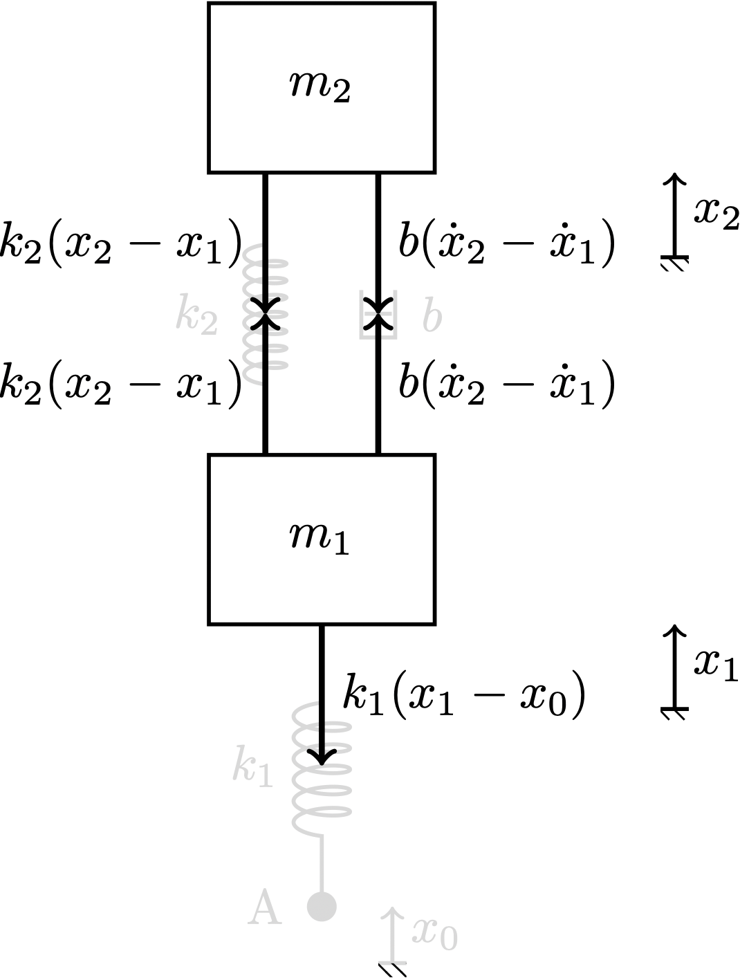
From the free body diagrams for this system we can write the following two equations representing Newton’s second law:

From the FBD of mass 1: \[m_1 \ddot{x}_1 = k_2(x_2-x_1) + b (\dot{x}_2-\dot{x}_1) - k_1 (x_1-x_0) \]
From the FBD of mass 2: \[m_2 \ddot{x}_2 = -k_2 (x_2-x_1) - b (\dot{x}_2-\dot{x}_1)\]

Rearranging this to get derivatives of the state variables, we can write

\[ \begin{aligned} \ddot{x}_1 &= \frac{k_2}{m_1}\left( x_2-x_1\right) + \frac{b}{m_1} \left( \dot{x}_2-\dot{x}_1 \right) - \frac{k_1}{m_1} \left( x_1-x_0\right) \\ \ddot{x}_2 &= -\frac{k_2}{m_2} \left( x_2-x_1 \right) - \frac{b}{m_2} \left( \dot{x}_2-\dot{x}_1 \right) \end{aligned} \]

Which then leads us to the state-variable equation

\[ \frac{d}{dt} \begin{bmatrix} x_1 \\ \dot{x}_1 \\ x_2 \\ \dot{x}_2 \end{bmatrix} = \begin{bmatrix} 0 & 1 & 0 & 0 \\ \displaystyle \left( -\frac{k_1}{m_1} - \frac{k_2}{m_1} \right) & \displaystyle -\frac{b}{m_1} & \displaystyle \frac{k_2}{m_1} & \displaystyle \frac{b}{m_1} \\ 0 & 0 & 0 & 1 \\ \displaystyle \frac{k_2}{m_2} & \displaystyle \frac{b}{m_2} & \displaystyle -\frac{k_2}{m_2} & \displaystyle -\frac{b}{m_2} \end{bmatrix} \cdot \begin{bmatrix} x_1 \\ \dot{x}_1 \\ x_2 \\ \dot{x}_2 \end{bmatrix} + \begin{bmatrix} 0 \\ \displaystyle \frac{k_1}{m_1} \\ 0 \\ 0 \end{bmatrix} \cdot \begin{bmatrix} \phantom{a} \\ x_0 \\ \phantom{a} \end{bmatrix} \]

The output equation should give us the two outputs as a linear combination of the state variables and the inputs, if applicable. In this case, the output equation is

\[ \boldsymbol{y} = \begin{bmatrix} k_2 & b & -k_2 & - b \\ -1 & 0 & 1 & 0 \end{bmatrix} \cdot \begin{bmatrix} x_1 \\ \dot{x}_1 \\ x_2 \\ \dot{x}_2 \end{bmatrix} + \begin{bmatrix} 0 \\ 0 \end{bmatrix} \cdot \begin{bmatrix} \phantom{a} \\ x_0 \\ \phantom{a} \end{bmatrix} \]

3.2 Step and Impulse Response

Use MATLAB to make plots of the step and impulse response of this system. Comment on the graphs by writing a short (two-to-three sentence) description of what the graphs show by referring to Figure 4. Use the following values for your parameters.

m1 = 10;
m2 = 4;
k1 = 5;
k2 = 5;
b  = 10;

Solutions

The following MATLAB code was used.

m1 = 10;
m2 = 4;
k1 = 5;
k2 = 5;
b = 10;

A = [0,                 1,      0,  0;
     -k1/m1-k2/m1,  -b/m1,  k2/m1,  b/m1;
     0,                 0,      0,  1;
     k2/m2,          b/m2, -k2/m2, -b/m2];

B = [0;
     k1/m1;
     0;
     0];

C = [k2, b, -k2, -b;
    0,  0, 1, 0];

D = [0;
    0];

sys=ss(A,B,C,D);

sys.OutputName = {'Force on m2','Position of m1'};

figure(1); clf;
step(sys);
saveas(gcf,"vibisol-stepresponse.png");
clf;
impulse(sys);
saveas(gcf,"vibisol-impulseresponse.png");

3.2.1 Step Response

The step response refers to how this system behaves if the massless point A is suddenly moved upward and kept there. From MATLAB, we find the step response to be the following.

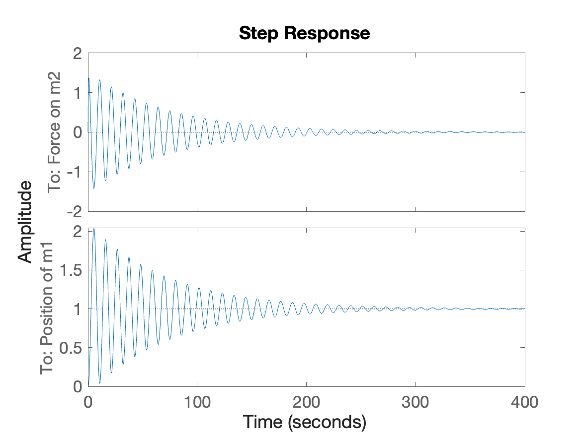
We see that the position of \(m_1\) moves up, oscillates about 1, and then settles down to 1. Since this is a unit step input, this means that the mass \(m_1\) moves up, in the end, just as much as we move the point A.

The force on \(m_2\) experiences some oscillations as the spring \(k_2\) and the damper \(b\) exert forces on it, but eventually these forces die out for a total force of zero.

3.2.2 Impulse Response

The impulse response refers to how this system behaves if the massless point A is suddenly moved upward and then brought back down.

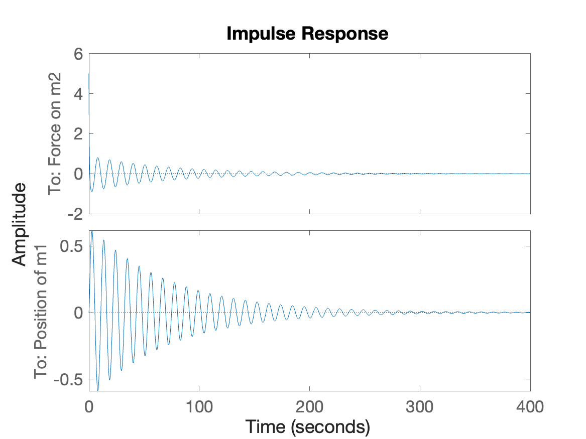
We see that the position of \(m_1\) moves up suddenly, but then comes back down to zero.

The force on \(m_2\) experiences significantly more oscillations than in the step response case, but once again the force dies down to zero eventually.