Numerically Solving Initial Value Problems

What is a numerical solution?

Initial Value Problems are not hard for a computer to solve. Typically, a computer uses a solution procedure that ‘marches forward in time’ starting from the initial condition and calculates subsequent values of \(x(t)\) in small increments of \(t\) until the entire domain of interest has been covered. The result is a collection of points of the form \[\{t_k, x_k \}, k = 1,2,3,... N\] instead of the usual \[x(t) = \text{ some function of } t.\]

Formatting differential equations for a computer

To communicate to a computer the initial value problem you want to solve, you must first write it in the form

\[\dot{x} = f(t,x)\] for a first-order differential equation. For now, we will not try to tackle higher-order differential equations.

A programming language of your choice

You have multiple options for how to solve initial value problems using a computer. We assume that you have already learned either MATLAB or Python, so you should become comfortable with at least one of the following approaches.

In the lectures and homework assignments, the emphasis will usually be on using numerical techniques to solve differential equations, not necessarily understanding how to write your own numerical solvers.

The exception to this is Lab 2, where you will learn to write a type of ode45 yourself.

For the purpose of these notes, though, the MATLAB function ode45 and the Python function scipy.integrate.solve_ivp will be treated as ‘black boxes’ that you will learn to use.

MATLAB

In MATLAB, there is a built-in function called ode45 that must be used to solve initial value problems. This does not need to be ‘loaded’ and comes pre-installed.

Read the documentation for how to use ode45 here.

Python

In Python, you must download and install the package scipy before you can solve initial value problems. Use pip install scipy to do this. You must write from scipy.integrate import solve_ivp at the top of every Python script where you want to use the function solve_ivp.

Read the documentation for how to use scipy.integrate.solve_ivp here.

Mathematica

In Mathematica, to which you have access as a Swarthmore student, initial value problems can be solved using the NDSolve function.

Read the documentation for how to use NDSolve here.

Code for solving a sample initial value problem

Consider the following IVP

\[ \dot{x} + x = t, \quad x(0) = 3 \tag{1}\]

whose solution can be determined by direct integration. (Try it!) Here, we will instead solve it numerically.

Python

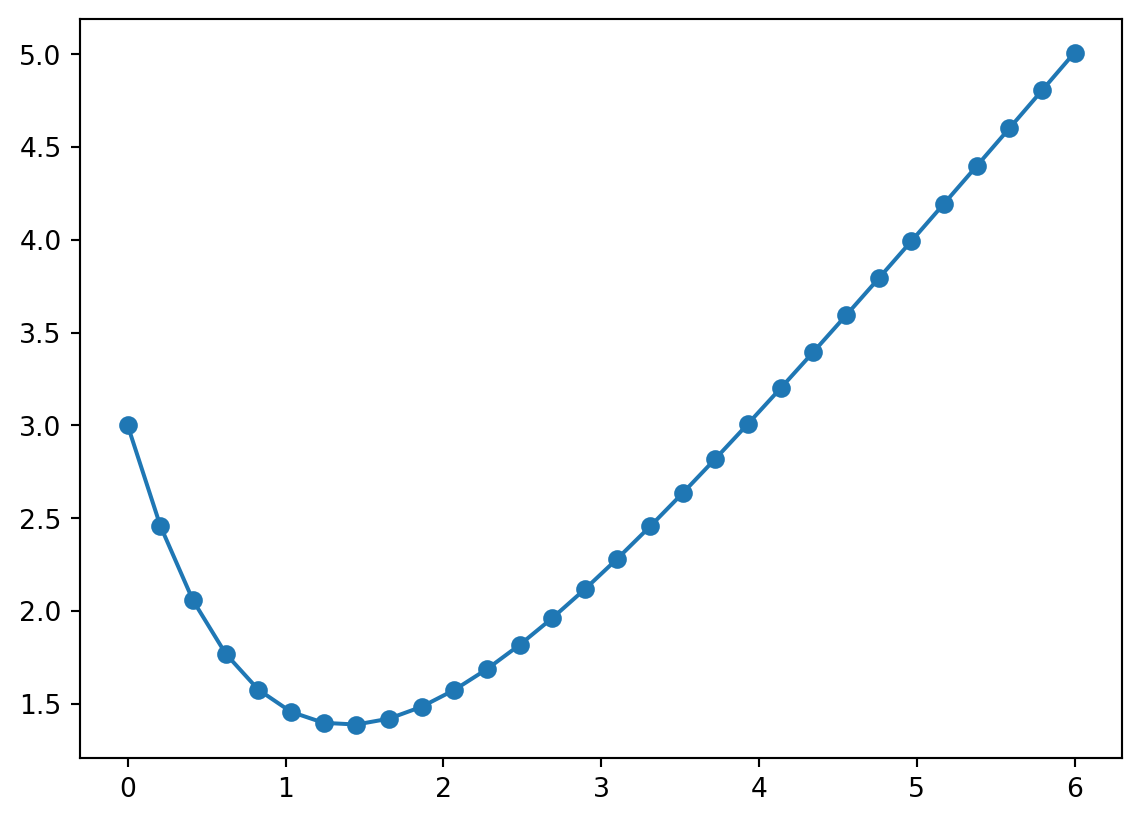
The following code can be adapted to solve any first-order differential equation numerically using Python. Here, we use it for Equation 1 specifically.

import numpy as np
import matplotlib.pyplot as plt
from scipy.integrate import solve_ivp

# Define a function that returns the value of f(t,x) for Equation 1.
def rhs1(t,x):
    return t - x[0]

# Define the values of t for which you care about the solution:
ts = np.linspace(0,6,30)

# Call 'solve_ivp' and assign the result to 'sol'
sol = solve_ivp(rhs1,   # first argument is the right-hand-side
                [0,6],  # second argument is the time span
                [3],      # third argument is the initial condition
                t_eval=ts # optional keyword argument
                )

# Plot the solution
plt.plot(ts, sol.y[0],'o-')
plt.show()

Note the following peculiarities of the syntax.

• The [0] on line 7: this tells Python to use the first element of x, which is assumed to be an array. For our purposes, this ‘array’ has size 1, i.e., x is really a scalar, but scipy.integrate.solve_ivp expects it to be an array, so the [0] is necessary.
• The initial condition has to be provided as an array, even if it’s a scalar as is the case here. That’s why we use [3], not 3
• The keyword argument t_evals=<something you specify> is optional, but bad things happen if you don’t use it.
• The result of solve_ivp is a custom Python object that has many attributes detailing how the solution turned out. Of these, the most important attribute is:
  • y, i.e., sol.y if you assigned the result of solve_ivp to something called sol. This contains the solution \(y(t)\) to the differential equation \(\dot{y} = f(t,y)\) in the form of a 1 x N array where N is the number of time-values at which the solution was found.
  • t, i.e., sol.t if you assigned the result of solve_ivp to something called sol. This contains the values of time at which the solution was calculated and stored. If you provide the keyword argument t_eval, sol.t will be equal to t_eval. For scalar problems such as Equation 1, the size of sol.t is the same as the size of sol.y.

MATLAB

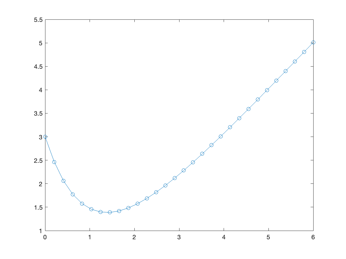
The following code can be adapted to solve any first-order differential equation numerically using MATLAB. Here, we use it for Equation 1 specifically.

numerical_solution.m

function dxdt = rhs1(t,x)
    % return the value of f(x,t)
    dxdt = t - x;
end

% Time span over which to integrate
tspan = linspace(0,6,30);

x0 = 3;

% Call ode45 and assign solution to x.
[t,x] = ode45(@rhs1, tspan, x0);

% Plot
plot(t, x, 'o-')

MATLAB result

Mathematica

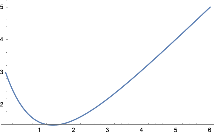
The following code can be adapted to solve any first-order differential equation numerically using Mathematica. Here, we use it for Equation 1 specifically.

numerical_solution.nb

sol = NDSolve[{x'[t] + x[t] == t, x[0] == 3}, x[t], {t, 0, 6}]
Plot[x[t] /. sol, {t, 0, 6}]

MATLAB result