Problem Set 10 Solutions
ENGR 12, Spring 2026.
Solutions
1 Making Bode Plots
1.1 Programmatically
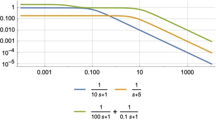
Draw the Bode plots (magnitude only) for the following systems on the same set of axes:
- \(\displaystyle T(s) = \frac{1}{10 s + 1}\)
- \(\displaystyle T(s) = \frac{1}{s + 5}\)
- \(\displaystyle T(s) = \frac{1}{0.1s+1}+ \frac{1}{100s+1}\)
You may wish to use the code provided on the resources page. You do not need to submit your code.
1.2 Sketching
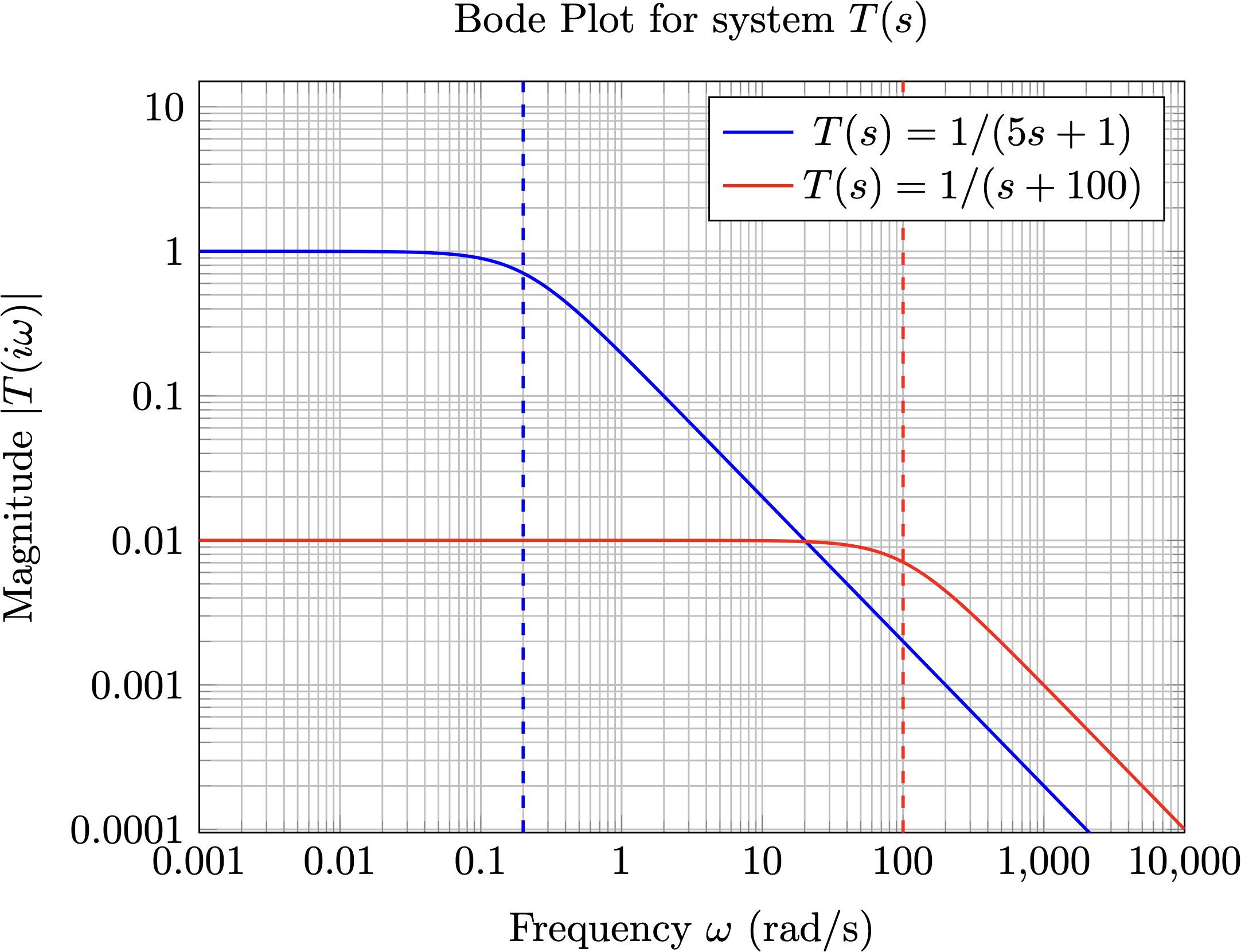
Sketch the Bode plots (magnitude only) for the following systems on the given set of axes. Label the corner frequency (in radians per second) for each case using a vertical line, and give its numerical value.
- \(\displaystyle T(s) = \frac{1}{s+100}\)
- \(\displaystyle T(s) = \frac{1}{5s + 1}\)
2 Plotting \(T(i \omega)\) on the complex plane for multiple transfer functions
We have learned that the complex number \(T(i \omega)\), where \(T(s)\) is the transfer function of a system, tells us about the amplitude ratio and phase shift of the steady-state response of that system relative to a sinusoidal input provided to it.
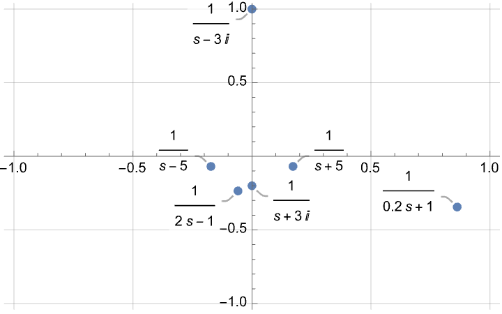
For the following transfer functions, plot \(T(i \omega)\) on the complex plane (i.e., put \(\mathrm{Re} T(i \omega)\) on the horizontal axis and \(\mathrm{Im} T(i \omega)\) on the vertical axis). Use \(\omega = 2\). You must put all of your points (six in total) on the same pair of axes, and you must label them with the transfer function expressions, either using ‘callouts’ or using a legend.
You can replace the plot with a very neatly-drawn and (within reason) quantitatively accurate sketch, if you prefer.
You may use a computer to help you with these calculations, but on a test you will be expected to this “by hand” with only a handheld calculator, if that. So it’s best to work this out manually.
- \(\displaystyle T(s) = \frac{1}{s+5}\)
- \(\displaystyle T(s) = \frac{1}{s-5}\)
- \(\displaystyle T(s) = \frac{1}{0.2s+1}\)
- \(\displaystyle T(s) = \frac{1}{2s-1}\)
- \(\displaystyle T(s) = \frac{1}{s+3i}\)
- \(\displaystyle T(s) = \frac{1}{s-3i}\)
3 Plotting \(T(i \omega)\) on the complex plane for multiple values of \(\omega\).
Consider the transfer function
\[T(s) = \frac{1}{5 s+1}, \tag{1}\]
subjected to sinusoidal inputs of unit magnitude and angular frequency equal to \(\{ 0.01, 0.1, 0.2, 2, 10 \}\).
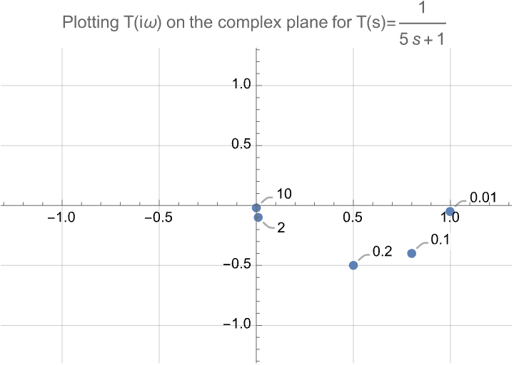
3.1 On the complex plane
Plot \(T(i \omega)\) for each of the above values of \(\omega\) on the complex plane.
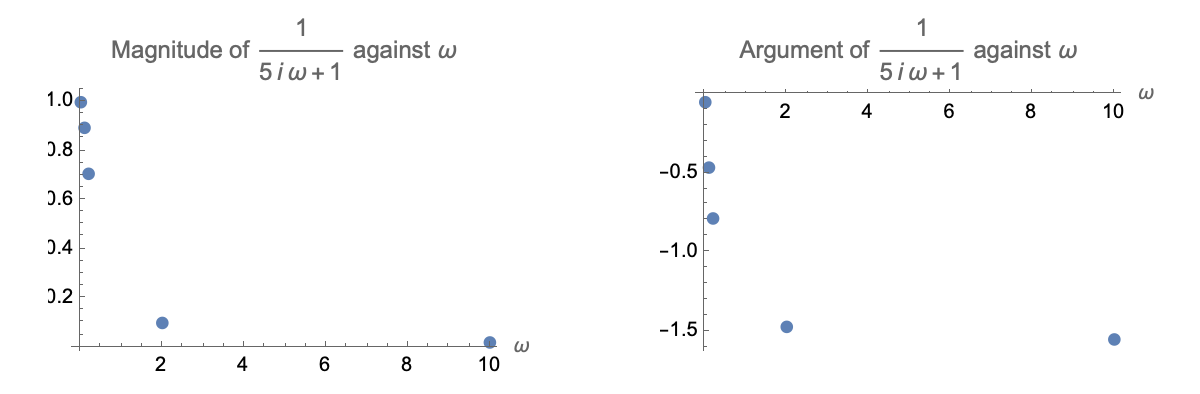
3.2 Plotted against \(\omega\)
Plot \(|T(i\omega)|\) and \(\angle T(i \omega)\) against \(\omega\) for the five values of \(\omega\) given above. There will be a total of two plots, and each plot will have five data points only. You may or may not choose to connect your five points with a curve or lines.
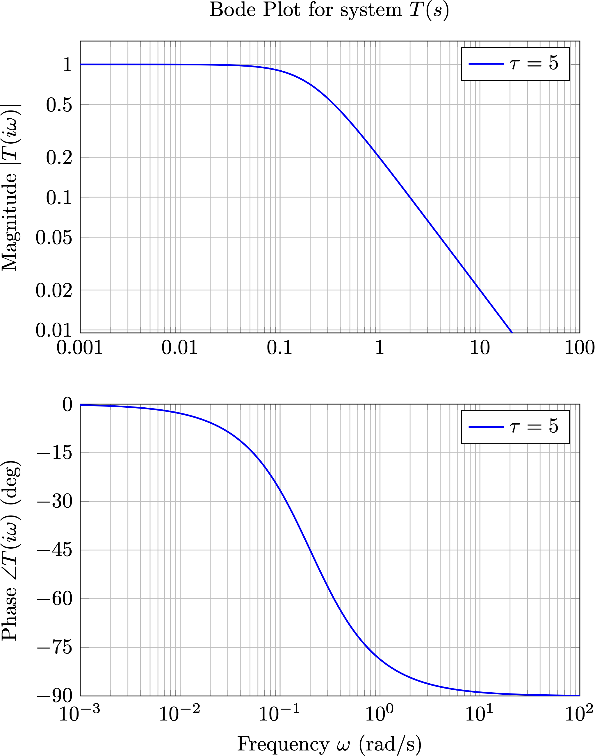
3.3 Bode Plot
Draw the Bode plot for the system given by Equation 1. You may choose to use plotting software, or sketch a quantitatively accurate graph on the following set of axes. In either case, use the given axis limits and grid markings.
4 Amplitude Ratio and Phase Shift
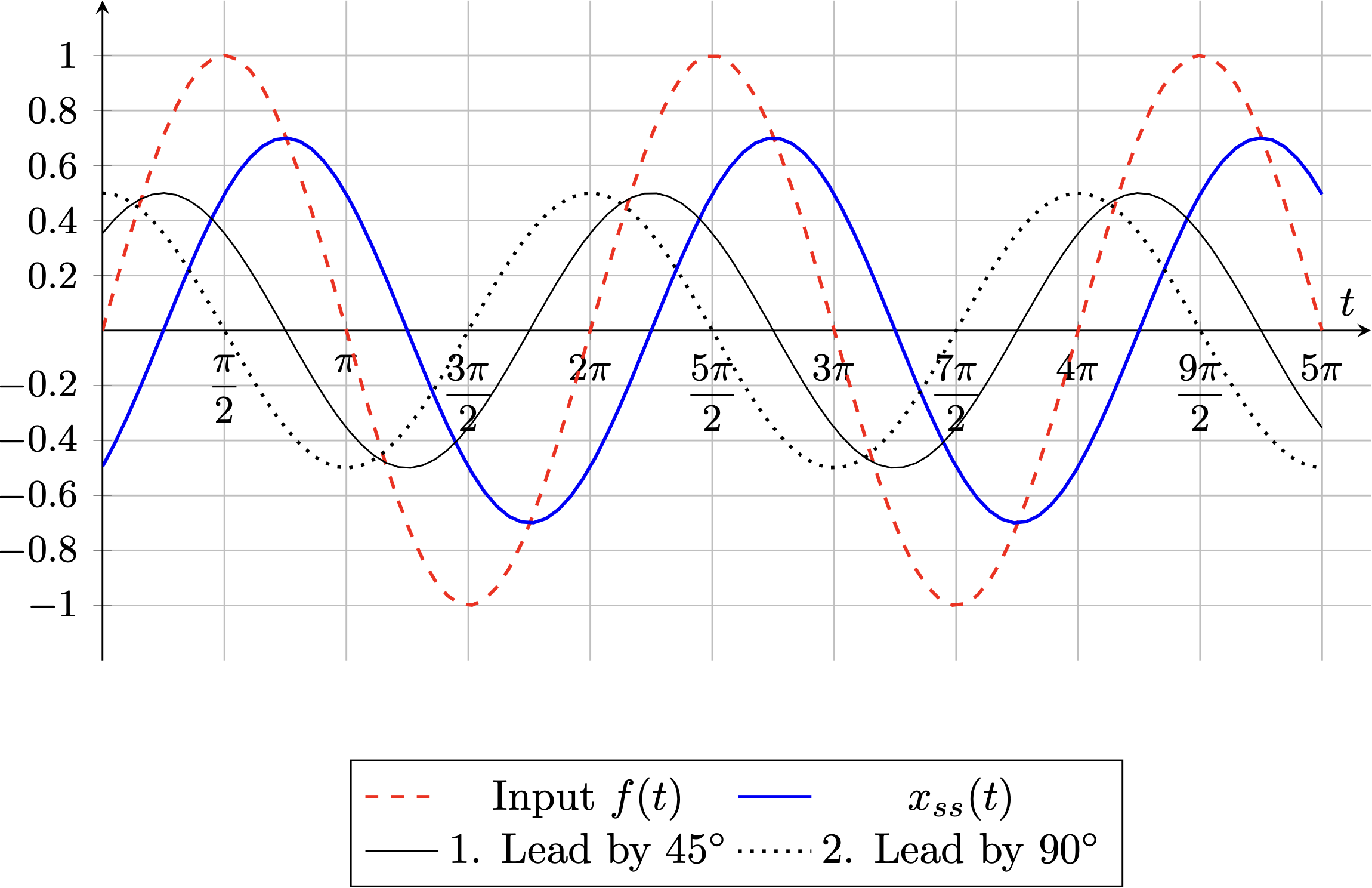
A certain linear system has input \(f(t)\) as shown in the graph below, and the corresponding steady state output \(x_{ss}(t)\), also shown on the same axes.
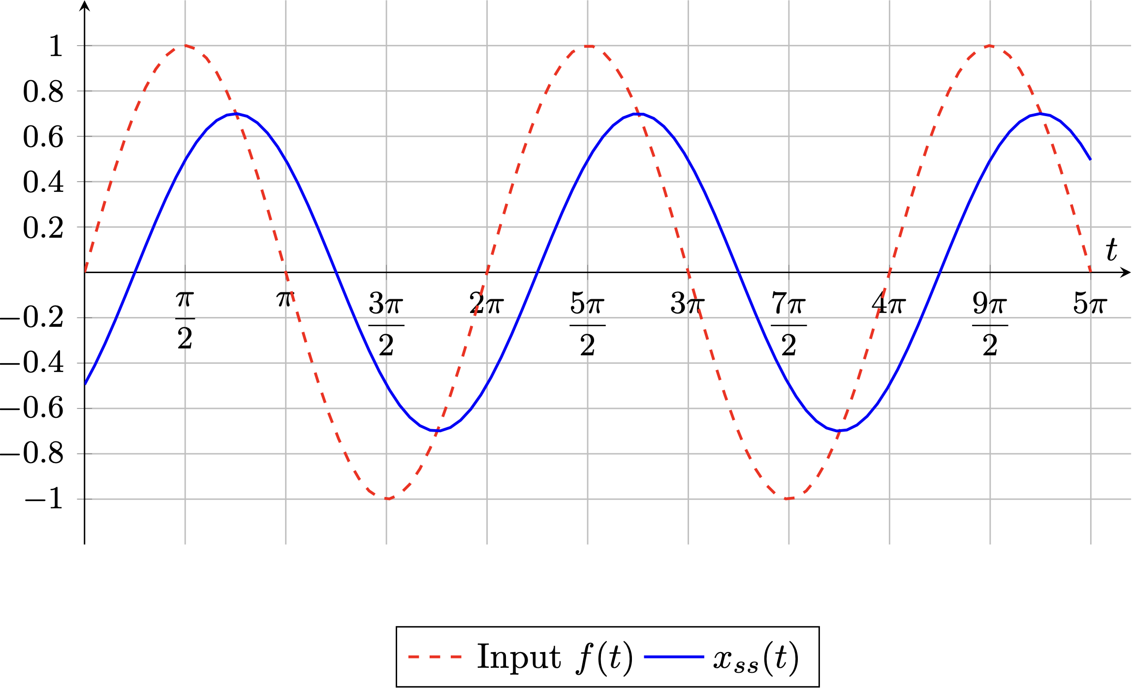
The transients, if any, are not shown in this graph.
4.1 Order of the system
Determine, if possible, the order of this system.
In this class we have seen that both first- and second-order systems subjected to a sinusoidal input will give a sinusoidal output.
4.2 Magnitude and argument of \(T(i\omega)\)
The magnitude of a complex number \(z\) is denoted by the symbol \(|z|\) or sometimes \(\text{abs}(z)\). The argument of a complex number \(z\) is denoted by the symbol \(\angle z\) or \(\arg z\).
If the transfer function for this system is given by \(T(s)\), determine the magnitude and argument of \(T(i \omega)\) for \(\omega = 1\). Present this information visually in the form of a complex plot, where the real part of \(T(i\omega)\) is shown on the horizontal axis and the imaginary part of \(T(i\omega)\) is shown on the vertical axis. You must also give the numerical values of \(|T(i \omega)|\) and \(\angle T(i \omega)\).
This question asks you to visually interpret Figure 1. For the vertical axis, read the graph to the closest half-interval, and for the horizontal axis, read the graph in increments of \(15^{\circ}\). Do not give the answer in angles of greater than \(+180^{\circ}\) or less than \(-180^{\circ}\).
The amplitude of the graph is about \(0.7\) and it is shifted about 45 degrees to the right. This means that \[x_{\text{ss}}(t) = 0.7 \sin (\omega t - 45^{\circ})\] so we have \[|T(i\omega)| = 0.7, \quad \angle T(i \omega) = 45^{\circ}\] when \(\omega = 1\).
4.3 Identifying the Transfer Function
Which of the following could be the transfer function for this system?
Calculate \(|T(i\omega)|\) and \(\angle T(i \omega)\) for each transfer function and compare with the values you expect.
To answer this question, we find the argument and magnitude of \(T(i\omega)\) for each of these.
We find that
| \(T(s)\) | \(|T(i\omega)|\) at \(\omega = 2\) | \(\angle T(i\omega)\) |
|---|---|---|
| \(\displaystyle \frac{1}{s+i}\) | \(\displaystyle \frac{1}{\sqrt{(1+\omega^2)^2}} = \frac{1}{{2}} = 0.500\) | \(\displaystyle \tan^{-1} \left(-\frac{1/(1+\omega)}{0} \right) = - 90^{\circ}\) |
| \(\displaystyle \frac{1}{s+1}\) | \(\displaystyle \frac{1}{\sqrt{1+\omega^2}} = \frac{1}{\sqrt{2}} \approx 0.707\) | \(\displaystyle \tan^{-1} \left(-\frac{\omega}{1} \right) = - 45^{\circ}\) |
| \(\displaystyle \frac{1}{s+2}\) | \(\displaystyle \frac{1}{\sqrt{4+\omega^2}} = \frac{1}{\sqrt{5}} \approx 0.447\) | \(\displaystyle \tan^{-1} \left(-\frac{\omega}{2} \right) = -\tan^{-1} \frac{1}{2} \approx -0.463\) |
Thus, we find that the second option has an amplitude ratio close to \(0.7\) and a phase shift of \(-90^{\circ}\).
4.4 Lag vs. Lead
The situation in Figure 1 can be described in the following words: the output \(x(t)\) lags the input \(f(t)\) by [some number of degrees or radians]. This refers to the fact that a peak in \(f(t)\) occurs first, and after some time (known as the lag duration), a peak in \(x(t)\) occurs. The opposite of ‘to lag’ is ‘to lead’.
Sketch, on a copy of the graph shown, an output signal \(x_2(t)\) that has an amplitude ratio \(0.5\) and that leads the input signal \(f(t)\) by
- 90 degrees
- 45 degrees