Making Bode Plots

Code for Bode Plots

Python

import matplotlib.pyplot as plt
from numpy import ones_like, sin, cos, linspace, logspace, sqrt, abs, log10, arctan, pi

tau = 5
tau2 = 0.05
omega = logspace(-2,3,500)

M_values = 1/sqrt(1+(omega*tau)**2)
M_values2 = 1/sqrt(1+(omega*tau2)**2)

phi_values = - arctan(omega*tau)
phi_values2 = - arctan(omega*tau2)

fig, (ax1, ax2) = plt.subplots(2, 1, figsize=(8, 8))

# --- TOP SUBPLOT ---
ax1.loglog(omega, M_values, label=f"$\\tau = {tau}$")
ax1.loglog(omega, M_values2, label=f"$\\tau = {tau2}$")
ax1.set_title('First-order systems $\\tau \\dot{y} + y = f(t)$ ')
ax1.set_ylabel('Gain |Y|/|F|')
ax1.grid(True, which="both", ls="-", alpha=0.5)
ax1.legend(loc="lower left")
ax1.axhline(0, color='black')
#ax1.axvline(1/tau, color='red',ls='--')
#ax1.axvline(1/tau2, color='red',ls='--')

# --- BOTTOM SUBPLOT ---
ax2.semilogx(omega, phi_values, label=f"$\\tau = {tau}$")
ax2.semilogx(omega, phi_values2, label=f"$\\tau = {tau2}$")
ax2.set_xlabel('Frequency $\\omega$ (rad/s)')
ax2.set_ylabel('Phase Shift $\\phi$')
ticks = [0, -pi/12, -pi/6, -pi/4, -pi/3, -5*pi/12, -pi/2]
labels = ['0', r'$-15^{\circ}$', r'$-30^{\circ}$', r'$-45^{\circ}$', r'$-60^{\circ}$', r'$-75^{\circ}$', r'$-90^{\circ}$']
ax2.set_yticks(ticks)
ax2.set_yticklabels(labels)
ax2.grid(True, which="both", ls="-", alpha=0.5)
ax2.legend(loc="lower left")
ax2.axhline(0, color='black')

plt.tight_layout()

MATLAB

% --- Parameters ---
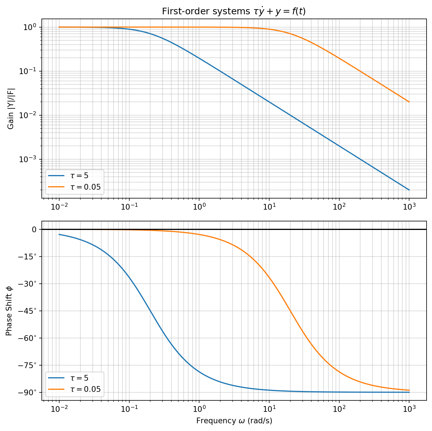
tau = 5;
tau2 = 0.05;
omega = logspace(-4, 4, 500);

% --- Calculations: You should only need to change this part---
M_values = 1 ./ sqrt(1 + (omega .* tau).^2);
M_values2 = 1 ./ sqrt(1 + (omega .* tau2).^2);

phi_values = -atan(omega .* tau);
phi_values2 = -atan(omega .* tau2);

% --- Initialize Figure ---
figure(1); clf;

% --- TOP SUBPLOT: Magnitude ---
ax1 = subplot(2, 1, 1);
loglog(omega, M_values, 'LineWidth', 2, 'DisplayName', ['$\tau = ', num2str(tau), '$']);
hold on;
loglog(omega, M_values2, 'LineWidth', 2, 'DisplayName', ['$\tau = ', num2str(tau2), '$']);
% Use LaTeX for Title and Labels
title('First-order systems $\tau \dot{y} + y = f(t)$', 'Interpreter', 'latex', 'FontSize', 20);
ylabel('Gain $|Y|/|F|$', 'Interpreter', 'latex', 'FontSize', 18);
grid on; grid minor;
ylim(ax1, [10^-4, 5]);

% Fix Legend Interpreter
lgd1 = legend('Location', 'southwest');
set(lgd1, 'Interpreter', 'latex', 'FontSize', 16);

% --- BOTTOM SUBPLOT: Phase ---
ax2 = subplot(2, 1, 2);
semilogx(omega, phi_values, 'LineWidth', 2, 'DisplayName', ['$\tau = ', num2str(tau), '$']);
hold on;
semilogx(omega, phi_values2, 'LineWidth', 2, 'DisplayName', ['$\tau = ', num2str(tau2), '$']);

xlabel('Frequency $\omega$ (rad/s)', 'Interpreter', 'latex', 'FontSize', 18);
ylabel('Phase Shift $\phi$', 'Interpreter', 'latex', 'FontSize', 18);

% --- Custom Tick Handling with LaTeX ---
ticks = [-pi/2, -5*pi/12, -pi/3, -pi/4, -pi/6, -pi/12, 0];
labels = {'$-90^\circ$', '$-75^\circ$', '$-60^\circ$', '$-45^\circ$', '$-30^\circ$', '$-15^\circ$', '$0^\circ$'};

set(ax2, 'YTick', ticks,'YTickLabel', labels,'TickLabelInterpreter', 'latex');

grid on; grid minor;
lgd2 = legend('Location', 'southwest');
set(lgd2, 'Interpreter', 'latex', 'FontSize', 16);