Higher-Order Initial Value Problems
Files for download
The following MATLAB scripts solve the equation \[m \ddot{x} + kx = f(t)\] for three different choices of \(f(t)\).
Solving the equation \[m \ddot{x} + k x = 0\]
The second-order differential equation \[m \ddot{x} + k x = 0\] with initial conditions \(x(0) = x_0, \dot{x}(0) = v_0\) is known to have the solution \[x(t) = x_0 \cos \omega t + \frac{v_0}{\omega} \sin \omega t\] where \(\omega^2 = k/m\).
To solve this Initial Value Problem in MATLAB, we set up the equation in the form
\[\frac{d}{dt} \begin{bmatrix} y_1 \\ y_2 \end{bmatrix} = \begin{bmatrix} y_2 \\ - (k/m) y_1 \end{bmatrix} \] where we have used the mapping \(x \rightarrow y_1\) and \(\dot{x} \rightarrow y_2\).
In MATLAB, the above function can be described using the following code, with some suitable numerical values for \(k = 5\) and \(m=3\).
function dydt = rhs(t,y)
% Implements the right-hand-side of the equation
% dy/dt = f(y,t)
% where y is a vector containing n state variables.
% Here, we are interested in the equation m x'' + k x = 0
% So y1 = x and y2 = x'.
    % un-pack contents of y
    y1 = y(1);
    y2 = y(2);

    % define constants
    k = 5; m = 3;

    % Define what dy/dt is
    dy1dt = y2;
    dy2dt = -(k/m)*y1;

    % Assemble contents of dy/dt into a column vector
    dydt = [dy1dt;dy2dt];
end
The above function can then be used in the following way to generate a solution to the IVP.
% Use ode45 from t = 0 to t = 10. Initial conditions are
% x(0) = 1, x'(0) = 0
[t,ysol] = ode45(@rhs,[0,10],[1;0]);

% Make plot
plot(t,ysol); % Plots both columns of 'ysol' in one go
legend("x","x dot","Location","southeast");

% Format plot nicely
set(0, 'DefaultLineLineWidth', 2);
set(gca,"FontName","EB Garamond");
set(gca,"LineWidth",1);
xlabel("Time [seconds]");
ylabel("Position or Velocity");
set(gca,"FontSize",20);
grid on;

% Save it
saveas(gcf,"MATLABfig1.png")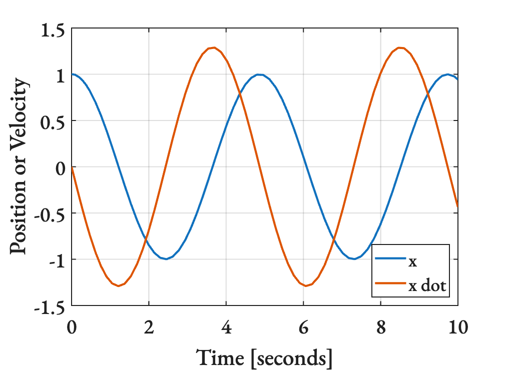
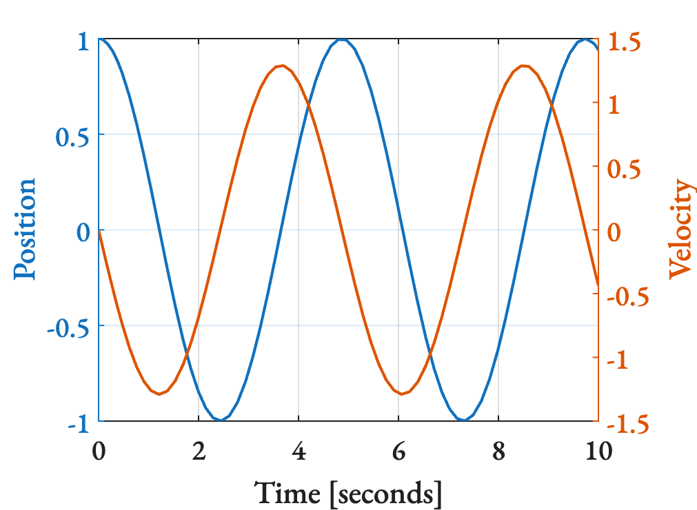
An alternative way to plot the same information by using two axes, one for the left and one for the right, is shown below.
% Use ode45 from t = 0 to t = 10
[t,ysol] = ode45(@rhs,[0,10],[1;0]);

% Unpack contents of ysol
pos = ysol(:,1); % x
vel = ysol(:,2); % x-dot

% Plot on the left
yyaxis left;
plot(t,pos);
ylabel("Position");

% Plot on the right
yyaxis right;
plot(t,vel);
ylabel("Velocity");

% Format plot nicely
set(0, 'DefaultLineLineWidth', 2);
set(gca,"FontName","EB Garamond");
set(gca,"LineWidth",1);
xlabel("Time [seconds]");
set(gca,"FontSize",20);
grid on;

% Save it
saveas(gcf,"MATLABfig2.png")