Problem Set 1
ENGR 12, Spring 2026.
| Due Date | Thu, Jan 29, 2026 |
| Turn in link | Gradescope |
| Latest version | Course website |
Note: 20% points on this assignment are for presentation and formatting of work.
1 Linearize a nonlinear ‘system’
Consider the nonlinear function \[f(x) = 5+x(x-4)(x-2) \tag{1}\]
Derive the expressions for a ‘linear model’ of Equation 1 near…
- \(x=1\)
- \(x=2\)
- \(x=4\)
As used in this assignment, the term ‘linear model’ refers to a function \(f^*(x)\) such that \(f(x)\) is approximately equal to \(f^*(x)\) in some part of the domain. \(f^*(x)\) should be linear in \(x\).
Write out your answers including your derivation by hand.
Neatly handwritten answers are expected here. You may choose to submit typed answers, but only if you use proper typesetting software like LaTeX.
Plot the functions that you find in the vicinity of each point, i.e., plot your answer to 1 in a small neighborhood of \(x=1\), your answer to 2 in a small neighborhood of \(x=2\), and your answer to 3 in a small neighborhood of \(x=4\). Overlay all three plots on a global plot of Equation 1 over a domain large enough to show the nonlinear behavior.
You may use any plotting software to do this; I recommend either matplotlib.pyplot in Python or the standard plotting commands in MATLAB. It is okay to use online resources to help you plot things, but your work must be your own.
If you need help getting started, check out the Resources page on the class website.
2 Complex Numbers
2.1 Cartesian and polar forms
The Cartesian form of a complex number is
\[z = x+iy, \tag{2}\]
and its polar form is
\[z = r e^{i \theta} \tag{3}\]
- Derive the polar form of the following complex numbers given in Cartesian form, i.e., calculate \(r\) and \(\theta\) and then write it in a form like Equation 3
- \(z_1 = 2 + 7i\)
- \(z_2 = -3 + 7i\)
- \(z_3 = -5 - 8i\)
- Derive the Cartesian form of the following complex numbers given in polar form, i.e., write it in the form of Equation 2.
- \(z_4 = 5e^{0.5i}\)
- \(z_5 = 5ie^{i \pi/6}\)
- \(z_6 = 3 e^{0}\)
2.2 Complex Arithmetic
Complex numbers can be added, subtracted, multiplied and divided.
Calculate the following complex numbers and give them in Cartesian or polar form.
- \[(-2)e^{0.3i} + 3 e^{5i}\]
- \[2+5i - e^{-i\pi/4}\]
- \[(5+i) \times (3-i)\]
- \[2e^{3i} \times (-9) e^{7i}\]
- \[(6+7i) \div (7-6i)\]
- \[-4e^{7i} \div 3 e^{5i}\]
2.3 Plotting Complex Numbers
Start with the complex number \(z_7 = 2 + 3i\). On the same set of coordinate axes representing the complex plane, plot
Remember that \(\bar{z}\) is the complex conjugate of \(z\), i.e., if \(z = x+ i y\) then \(\bar{z} = x - i y\).
- A point corresponding to \(z_7\).
- An arrow from the origin to \(z_7\).
- A point corresponding to \(i z_7\).
- An arrow from the origin to \(i z_7\).
- A point corresponding to \(-z_7\).
- An arrow from the origin to \(-z_7\).
- A point corresponding to \(\bar{z_7}\).
- An arrow from the origin to \(\bar{z_7}\)
3 Differential Equations
3.1 Placing equations in the standard form
The standard form for writing down a first-order differential equation is \[\dot{x} = f(x,t). \tag{4}\]
Place the following equations in the form of Equation 4. In doing so, explicitly identify and write down the function \(f(x,t)\).
Remember that \[f(x,t)\] could be a constant, just a function of \(t\), just a function of \(x\), or a function of \(both\).
- \[\dot{x} + 2x = 1/x\]
- \[\dot{x}^2 + 2x = t\]
- \[\dot{x}x + 2 = \cos t\]
- \[\dot{x} = e^x - e^t\]
- \[\dot{x} + \cos(t) x = 5\]
- \[\dot{x} = \frac{1}{x}\]
3.2 Coupled and uncoupled differential equations
Which of the following sets of equations are coupled? State whether the coupling is in both ways, or only one way, and if the latter, then specify which way it is coupled. You do not need to show your work for this.
\[ \begin{aligned} m_1 \frac{d v_1}{dt} + b_1 v_1 &= 0 \\ m_2 \frac{d v_2}{dt} + b_2 v_2 &= 0 \end{aligned} \tag{5}\]
\[ \begin{aligned} m_1 \frac{d v_1}{dt} + b_1 v_1 &= 0 \\ m_2 \frac{d v_2}{dt} + b_2 (v_2-v_1) &= 0 \end{aligned} \tag{6}\]
\[ \begin{aligned} m_1 \frac{d v_1}{dt} + b_1 (v_1-v_2) &= 0 \\ m_2 \frac{d v_2}{dt} + b_2 v_2 &= 0 \end{aligned} \tag{7}\]
\[ \begin{aligned} m_1 \frac{d v_1}{dt} + b_1 (v_1-v_2) &= 0 \\ m_2 \frac{d v_2}{dt} + b_2 (v_2-v_1) &= 0 \end{aligned} \tag{8}\]
3.3 Linear and nonlinear differential equations
Which of the following differential equations are linear and which are nonlinear?
A differential equation is linear if the function \(f\) appearing on its right-hand side is linear in \(x\) and all its derivatives
- \[2 \dot{x} + x = \cos t\]
- \[(\dot{x} + x) \cos x = t\]
- \[(\dot{x} + x) \cos \pi/6 = 2t \]
- \[\dot{x} = \frac{1}{x} \]
- \[\ddot{x} + 2 \dot{x}^2 - 3x = 2t \]
- \[\ddot{x} + 2 \dot{x} - 3x = 2t \]
4 A coupled first-order linear system
is not necessary for this problem. We haven’t gotten to that yet! The plots shown below were made by a computer program. Very soon, you’ll learn how to make them yourself, but for now, don’t worry about how the solution was arrived at.
In class, we discussed the system described by the following diagram.

We will assume that the upper box is so much smaller than the lower box that it will never fall off. The lower box is assumed to be on the ground and the ground goes on for ever.
The governing equations for this system, if it’s not subjected to any external forces, are
\[ \begin{aligned} m_1 \dot{v}_1 &+ b_1 v_1 =0 \\ m_2 \dot{v}_2 &+ b_2 (v_2-v_1) = 0 \end{aligned} \]
If you start this system off such that the bottom box has a starting positive nonzero speed, while the top box starts off with zero speed, it can be shown that the speeds of the two boxes \(v_1\) and \(v_2\) (in the directions shown in the diagram) will evolve over time as follows.
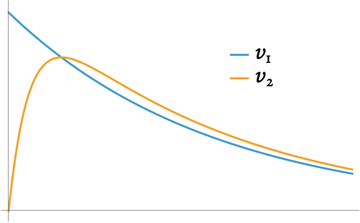
Note that box 1 is ten times heavier than box 2, and the two friction coefficients \(b_1\) and \(b_2\) are equal to each other.
4.1 Tasks
According to your intuition, what happens to the boxes’ positions as measured from the fixed wall? Will \(x_1\) and \(x_2\), measured relative to the wall, both increase? Or will one of them increase and the other decrease? Describe what happens to the boxes’ positions in a few sentences.
Using Figure 1, make a sketch of \(x_1\) and \(x_2\) as a function of time for the first few moments of the motion, until the orange and blue lines shown above intersect. Start both \(x_1\) and \(x_2\) from zero, which effectively means we’re re-defining zero to be wherever things started. Your knowledge of calculus will help you with this task. Remember that this is a qualitative, not a quantitative task.
Also make a sketch of \((x_2 - x_1)\) against time on the same set of axes as above, and explain what this represents physically.
The point where \(v_1\) and \(v_2\) intersect is where the two boxes have the same velocity, not position!