Lecture 14
E12 Linear Physical Systems Analysis
Examples of second-order systems with damping
Second-order systems with damping
The second-order differential equation \[\ddot{x} + a \dot{x} + b x = 0\] usually has the solution \(x(t) =e^{s t}\) where \(s\) satisfies the characteristic equation \[s^2 + a s + b = 0 \implies s_{1,2} = \frac{-a \pm \sqrt{a^2-4b}}{2}\]
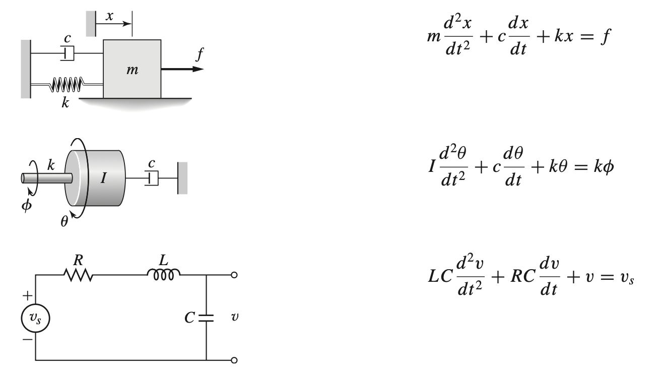
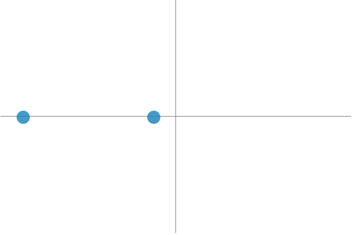
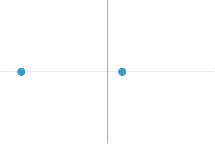
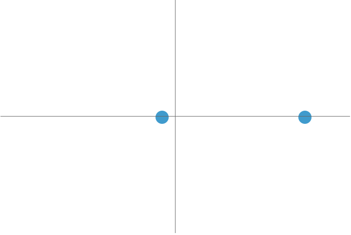
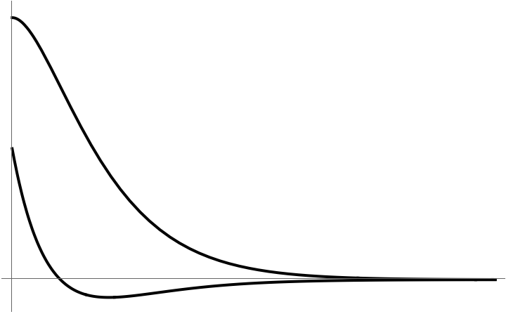
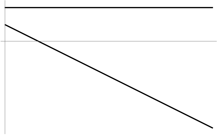
Case 1 when \(a^2 - 4b > 0\) and therefore \(s_{1,2} \in \mathbb{R}\)
\[x(t) = K_1 e^{s_1 t} + K_2 e^{s_2 t} \qquad K_1,K_2 \in \mathbb{R}\]
| Case 1a: \(s_1,s_2 < 0\) | Case 1b: \(s_1< 0<s_2\) | Case 1c: \(s_1, s_2 > 0\) |
|---|---|---|
| Both roots negative | One positive, one negative | Both roots positive |
 |
 |
 |
 |
 |
 |
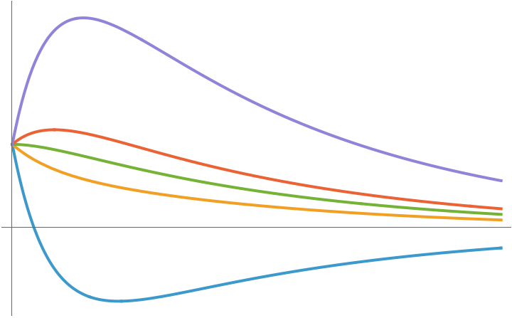
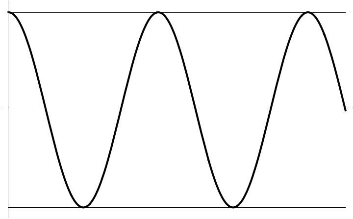
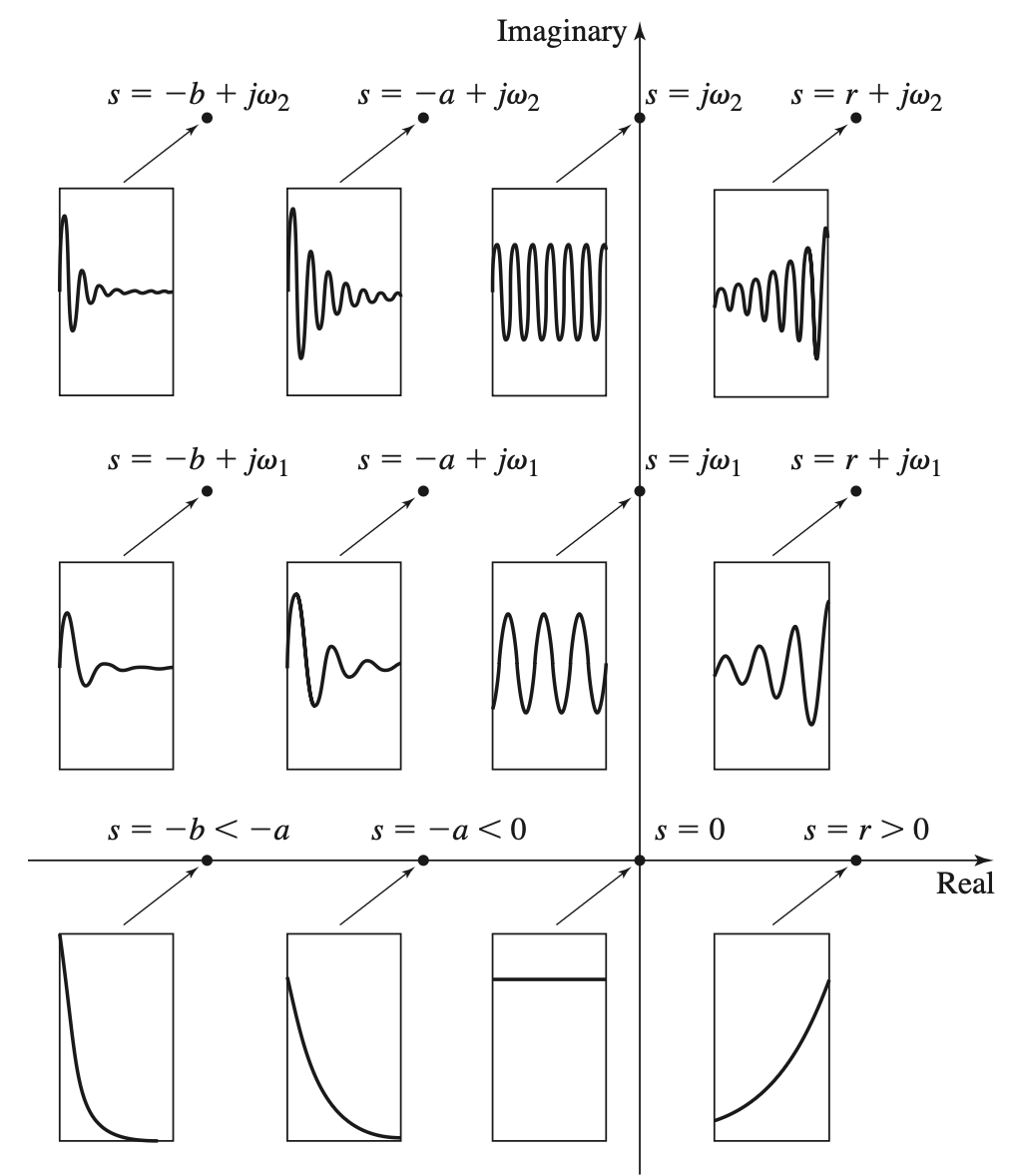
Case 2 when \(a^2 - 4b < 0\) and therefore \(s_{1,2} \in \mathbb{C}\)
\[ \begin{aligned} x(t) &= P e^{s_1 t} + \overline{P} e^{s_2 t} \qquad P \in \mathbb{C} \\ &= e^{rt} \left( A \cos \omega t + B \cos \omega t \right) \qquad A,B \in \mathbb{R} \\ s_{1,2} &= r \pm i \omega \end{aligned} \]
| Case 2a: \(r < 0\) | Case 2b: \(r = 0\) | Case 2c: \(r > 0\) |
|---|---|---|
| Real part negative | Real part zero | Real part positive |
 |
 |
 |
 |
 |
 |
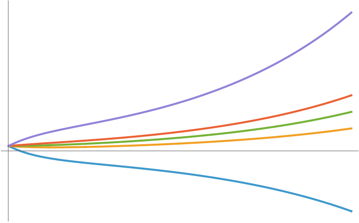
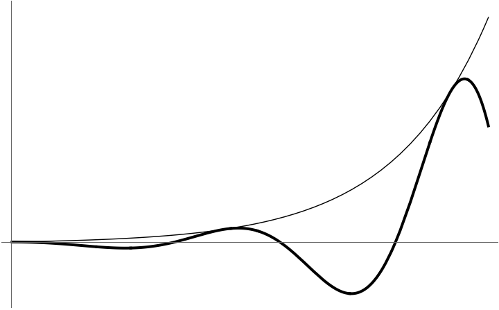
Case 3 when \(a^2 - 4b = 0\) and therefore \(s_1 = s_2\)
\[ x(t) = (C_1 + C_2t) e^{rt} \]
| Case 3a: \(r < 0\) | Case 3b: \(r = 0\) |
|---|---|
| Nonzero repeated roots | Repeated roots at zero |
 |
 |
 |
 |
Summary of 2nd-order systems with no input
The differential equation \[m \ddot{x} + b \dot{x} + k x = 0\]
admits solutions of the form \(e^{st}\) where \(s\) must be a root of the characteristic polynomial \[m s^2 + b s + k.\] The roots will, in general, be complex, and are given by \[s_{1,2} = \frac{-b \pm \sqrt{b^2-4mk}}{2m}.\] Then, the solution can usually be written as \[x(t) = A e^{s_1t} + B e^{s_2 t}\] where \(A\) and \(B\) are, in general, complex.
Case 1: Roots of characteristic polynomial are real
If \(b^2-4mk >0\), the two roots are real and are given by the real numbers \[s_{1,2} = \frac{-b \pm \sqrt{b^2-4mk}}{2m}\] and the solution can be written as \[\boxed{x(t) = K_1 e^{s_1 t} + K_2 e^{s_2 t}} \qquad \text{with }K_1,K_2,s_1,s_2 \in \mathbb{R}\]
Case 2: Roots of characteristic polynomial are complex
If \(b^2-4mk <0\), the two roots are complex and are given by the complex numbers \[ s_{1,2} = \frac{-b \pm \sqrt{b^2-4mk}}{2m} = r \pm i \omega, \] \[ \text{ where } \quad r = -\frac{b}{2m}, \quad \omega = \frac{1}{2m}\sqrt{4mk-b^2}\] and the solution can be written as \[x(t) = P e^{s_1 t} + \overline{P} e^{s_2 t} \qquad \text{with }P,s_1,s_2 \in \mathbb{C}\] or, alternatively, as \[\boxed{x(t) = e^{rt} \left( K_3 \cos \omega t + K_4 \sin \omega t \right)} \qquad \text{with }K_3,K_4,r,\omega \in \mathbb{R}\] or, alternatively, as \[x(t) = e^{rt} C_1 \cos \left( \omega t + \phi_1 \right) \qquad \text{with }C_1,\phi_1,r,\omega \in \mathbb{R}\] or, alternatively, as \[x(t) = e^{rt} C_2 \sin \left( \omega t + \phi_2 \right) \qquad \text{with }C_2,\phi_2,r,\omega \in \mathbb{R}\]
Case 3: Roots of characteristic polynomial are repeated
If \(b^2-4mk =0\), the two roots are repeated \[ s_1 = s_2 = \frac{-b \pm \sqrt{{b^2-4mk}}}{2m} = -b/2m = r\] and the solution can be written as (take MATH 43/44 to see why) \[\boxed{x(t) = (C_3 + C_4t) e^{rt}} \qquad \text{with }C_3,C_4,r \in \mathbb{R}\]
Changing the damping
Let’s examine solutions to \[m \ddot{x} + b \dot{x} + k x = 0, \qquad x(0) = 1, \dot{x}(0) = 0\] With \(k=2\), \(m=3\), and \(b\) allowed to vary from \(0\) to \(6\).
| Value of \(b\) | Motion |
|---|---|
| \(0.0\) | 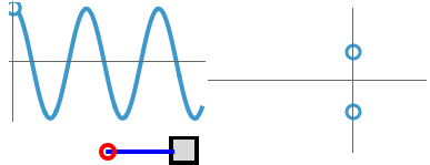 |
| \(0.5\) | 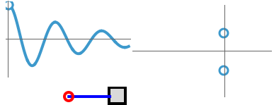 |
| \(1.0\) | 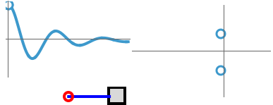 |
| \(1.5\) | 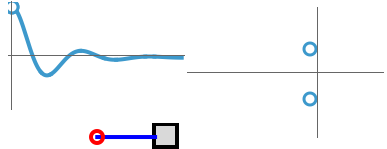 |
| \(2.0\) | 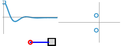 |
| \(2.5\) | 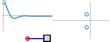 |
| \(3.0\) | 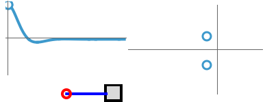 |
| \(3.5\) | 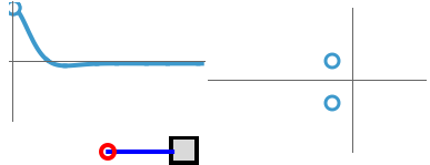 |
| \(4.0\) |  |
| \(4.5\) | 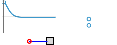 |
| \(5.0\) | 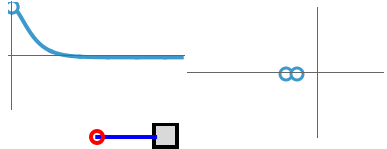 |
| \(5.5\) | 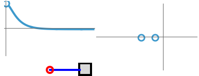 |
| \(6.0\) | 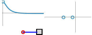 |
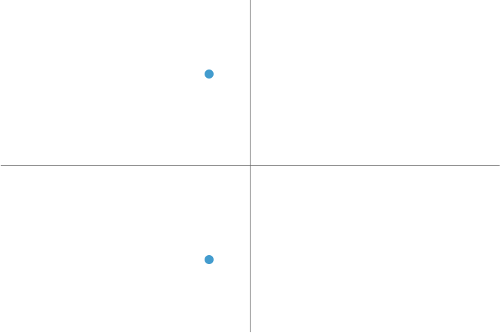
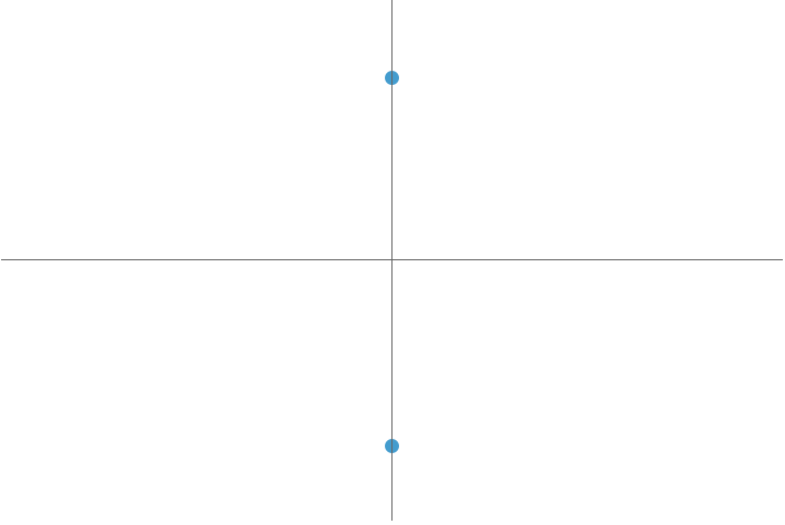
Effect of Root Location on free response
The system \(m \ddot{x} + b \dot{x} + kx = f(t)\) has a free response that depends on the roots of the characteristic polynomial \(m s^2 + b s + k\).
In general, these roots are complex, so we can plot them on the complex plane.
Critical Value of Damping
We’ve seen that something special happens when the damping coefficient \(b\) crosses some critical value. What is this critical value?
\(m \ddot{x} + b \dot{x} + kx = 0\) has the solutions \(e^{st}\) when \[m s^2 + b s + k = 0 \implies s = \frac{-b \pm \sqrt{b^2-4mk}}{2m}\]
- If \(b^2 - 4mk < 0\): \(\quad s_{1,2}\) has nonzero imaginary part (\(s_{1,2} \in \mathbb{C}\))
- If \(b^2 - 4mk > 0\): \(\quad s_{1,2}\) has zero imaginary part (\(s_{1,2} \in \mathbb{R}\))
- If \(b^2 - 4mk = 0\): \(\quad s_1 = s_2\) (repeated nonzero roots)
Recall that if — and only if — \(s \in \mathbb{C}\), then \(e^{st}\) will oscillate in time! (\(e^{i\theta} = \cos \theta + ...\))
There is a critical value of \(b = \sqrt{4mk}\) that demarcates qualitatively different behavior.
Introducing Damping Ratio
- There is a critical value of \(b = \sqrt{4mk}\) that demarcates qualitatively different behavior.
- Define a ratio \(\zeta\) (Greek letter ‘zeta’) \[\zeta = \frac{b}{\sqrt{4mk}}\] that is the ratio of damping parameter \(b\) to the critical damping parameter
Underdamped, overdamped, etc.
| Zeta \(\zeta\) | \(b\) | Name | Typical Motion and roots of \(m s^2 + b s + k\) |
|---|---|---|---|
| \(\zeta = 0\) | \(b=0\) | Undamped | |
| \(\zeta < 1\) | \(b < \sqrt{4mk}\) | Underdamped | |
| \(\zeta = 1\) | \(b = \sqrt{4mk}\) | Critically damped | 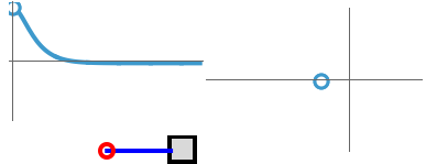 |
| \(\zeta > 1\) | \(b > \sqrt{4mk}\) | Overdamped | 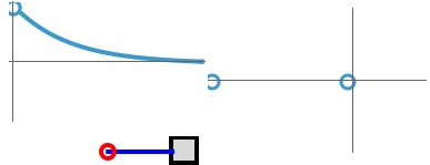 |
Governing equation for 2nd order system in terms of natural freqency and damping ratio
Recall that the natural frequency is given by \(\sqrt{k/m}\). From now on, we will call this the ‘undamped natural frequency’ and use the symbol \(\boxed{\omega_n}\).
\[ m \ddot{x} + b \dot{x} + kx = 0 \] \[ \phantom{m} \ddot{x} + \frac{b}{m} \dot{x} + \frac{k}{m}x = 0 \] \[ \phantom{m} \ddot{x} + \overbrace{\frac{{\color{green}{b}}}{m} \cdot \frac{\sqrt{m}}{{\color{green}{\sqrt{m}}}} \cdot \frac{\sqrt{k}}{{\color{green}{\sqrt{k}}}} \cdot \frac{2}{{\color{green}{2}}}}^{b/m} \dot{x} + \left(\frac{\sqrt{k}}{\sqrt{m}}\right)^2 x = 0 \] \[ \phantom{m} \ddot{x} + \frac{{\color{green}{b}}}{{\color{brown}{\sqrt{m}}}} \cdot \frac{{1}}{{\color{green}{\sqrt{m}}}} \cdot \frac{{\color{brown}{\sqrt{k}}}}{{\color{green}{\sqrt{k}}}} \cdot \frac{2}{{\color{green}{2}}} \dot{x} + \left(\frac{{\color{brown}{\sqrt{k}}}}{{\color{brown}{\sqrt{m}}}}\right)^2 x = 0 \] \[ {\color{green}{\frac{b}{2\sqrt{mk}}}} \text{ is the damping ratio } \zeta \] \[ {\color{brown}{\sqrt{\frac{k}{m}}}} \text{ is the undamped natural frequency } \omega_n \] \[ \implies \boxed{\ddot{x} + 2 {\color{green}{\zeta}}{\color{brown}{\omega_n}} x + {\color{brown}{\omega^2_n}} x = 0} \]
Damped vs. undamped natural frequency
We know that a system governed by \(m \ddot{x} + kx = 0\) has the free response \[ \begin{aligned} \textstyle x(t) &= \textstyle A \cos \left( t \sqrt{k/m} \right) + B \sin \left( t \sqrt{k/m} \right) \\ &= A \cos \omega_n t + B \sin \omega_n t \end{aligned} \] where \(A, B \in \mathbb{R}\) can be found using the initial conditions.
At what frequency does the system governed by \[m \ddot{x} + b \dot{x} + kx = 0 \tag{1}\] oscillate naturally?
- Same as \(\omega_n\) ?
- Faster than the undamped system?
- Slower than the undamped system?
Hint: Equation 1 is identical to \(\ddot{x} + 2 \zeta \omega_n x + \omega_n^2 x = 0\)
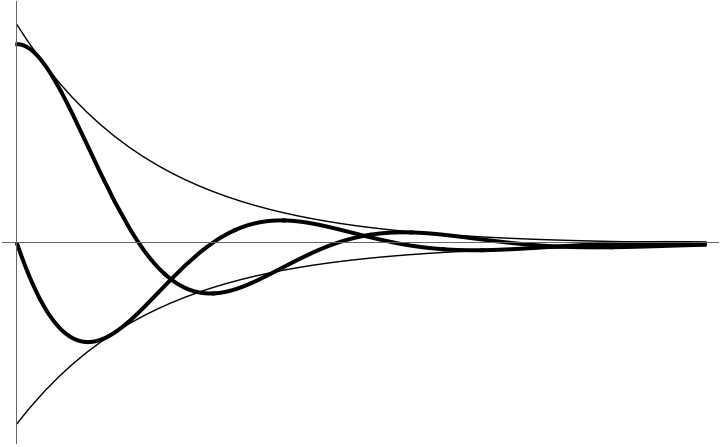
Damped Natural Frequency and Time Constant for second-order systems
Underdamped second order systems (with \(\zeta < 1\)) have a time constant that characterizes how quickly or slowly they decay.
Solutions are multiples of \(x(t) = e^{({\color{blue}{r}} \pm i {\color{brown}{\omega}} )t}\).
- \({\color{brown}{\omega}}\) is responsible for the oscillation
- \({\color{blue}{r}}\) is responsible for the decay
When \(m \ddot{x} + b \dot{x} + k x = 0\) is written in the form \[\ddot{x} + 2 \zeta \omega_n x + \omega_n^2 x = 0,\]
the roots of the characteristic polynomial \[s^2 + 2 \zeta \omega_n s + \omega_n^2\] are \[s = - \zeta \omega_n \pm i \omega_n \sqrt{1-\zeta^2}\]
with the solution for \(x(t)\) given by \[x(t) = e^{- {\color{blue}{\zeta \omega_n}}t} \left( A \cos \left( t\, {\color{brown}{\omega_n \sqrt{1-\zeta^2}}} \right) + B \sin \left( t\, {\color{brown}{\omega_n \sqrt{1-\zeta^2}}} \right) \right)\]
- \(\displaystyle {\color{blue}{\frac{1}{\zeta \omega_n}}}\) is known as the time constant
- \({\color{brown}{\omega_n \sqrt{1-\zeta^2}}}\) is known as the damped natural frequency
Step Response of a second-order system
Consider a spring-mass system starting from \(x = 0, \dot{x}=0\) that is subjected to a step function force \(f(t) = u_s(t)\)
\[\ddot{x} + 2 \zeta \omega_n \dot{x} + \omega_n^2 x = u_s(t)\]
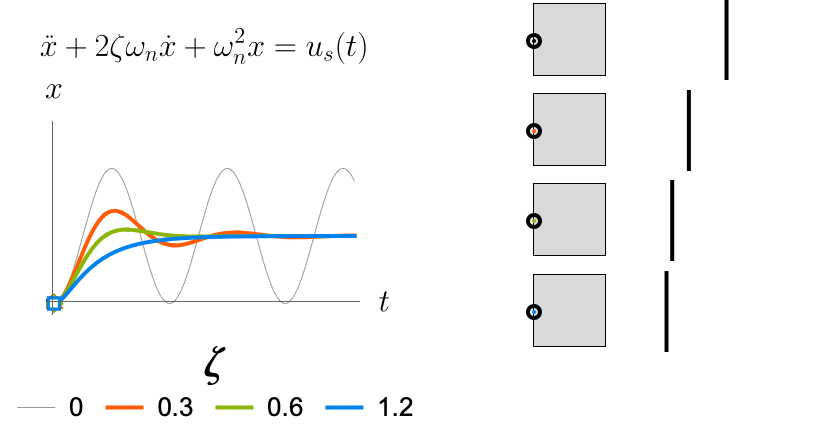
- When \(\zeta < 1\), overshoot occurs
- When \(\zeta > 1\), there’s no overshoot
Calculating the step response of a second-order system
Q. How does a spring-mass-damper system respond to a step-function force applied to it?
Approach:
- Write the differential equation
- Take Laplace Transform
- Solve for \(X(s)\)
- Use Inverse Laplace Transform to get \(x(t)\)
\[ m \ddot{x} + b \dot{x} + k x = u_s(t) \] \[ \mathcal{L}\left[ m \ddot{x} + b \dot{x} + k x \right] = \mathcal{L} \left[ u_s(t) \right] \] \[ m s^2 X + b s X + k X = \frac{1}{s} \] \[ \left( m s^2 + b s + k \right) X = \frac{1}{s} \] \[ X(s) = \frac{1}{s} \frac{1}{ m s^2 + b s + k} \]
Impulse Response of a second-order system
Consider a spring-mass system starting from \(x = 0, \dot{x}=0\) that is subjected to a impulse function force \(f(t) = \delta(t)\)
\[\ddot{x} + 2 \zeta \omega_n \dot{x} + \omega_n^2 x = \delta(t)\]
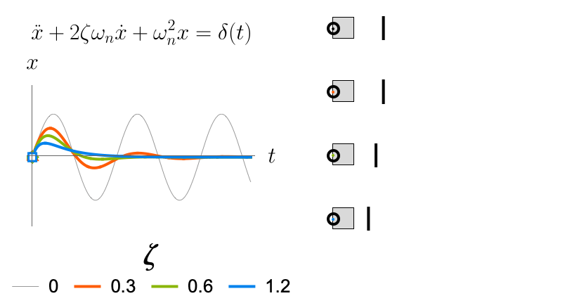
- When \(\zeta > 1\), no oscillations occur
- When \(\zeta < 1\), there’s oscillations
Calculating the impulse response of a second-order system
Q. How does a spring-mass-damper system respond to a Dirac Delta-function force applied to it?
Approach:
- Write the differential equation
- Take Laplace Transform
- Solve for \(X(s)\)
- Use Inverse Laplace Transform to get \(x(t)\)
\[ m \ddot{x} + b \dot{x} + k x = \delta(t) \] \[ \mathcal{L}\left[ m \ddot{x} + b \dot{x} + k x \right] = \mathcal{L} \left[ \delta(t) \right] \] \[ m s^2 X + b s X + k X = 1 \] \[ \left( m s^2 + b s + k \right) X = 1 \] \[ X(s) = \frac{1}{ m s^2 + b s + k} \]