Lecture 7

E12 Linear Physical Systems Analysis

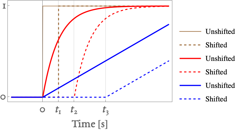
First-order systems’ response to pulse input

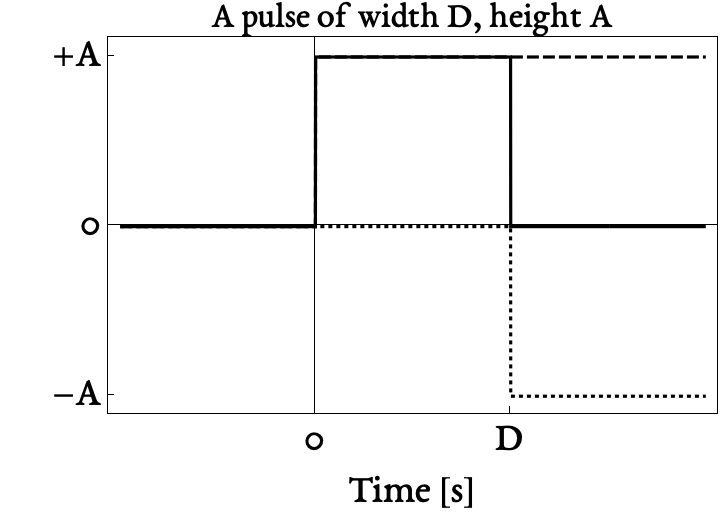
• What’s a pulse?

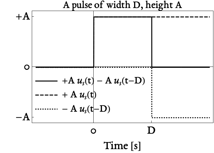
• A pulse can be constructed by superimposing scaled and shifted Heaviside Step Functions

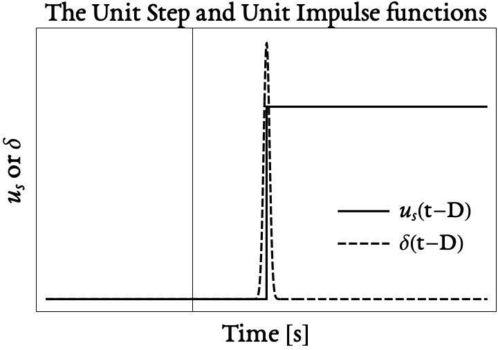
• Recall what those are: \[ u_s(t) = \begin{cases} 1 & t > 0 \\ 0 & t < 0 \end{cases} \]

• A pulse of width \(D\) and height \(A\) can be constructed using two (re-scaled and shifted) step functions

First-order systems’ response to pulse input

We wish to find \(x(t)\) when the input \(f(t)\) is the sum of two step functions. \[ \dot{x} + ax = \overbrace{A u_s(t) - A u_s(t-D)}^{f(t)} \]

• Approach: Use linearity!
• Separately find solutions of \(\dot{x} + ax = A u_s(t)\) and \(\dot{x} + ax = - A u_s(t-D)\), keeping \(x(0) = 0\).
• Add up the two solutions. This is the solution to \(\dot{x} + ax = f(t)\)

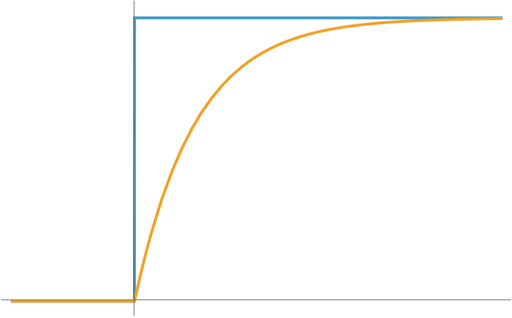
Step Response of First Order System

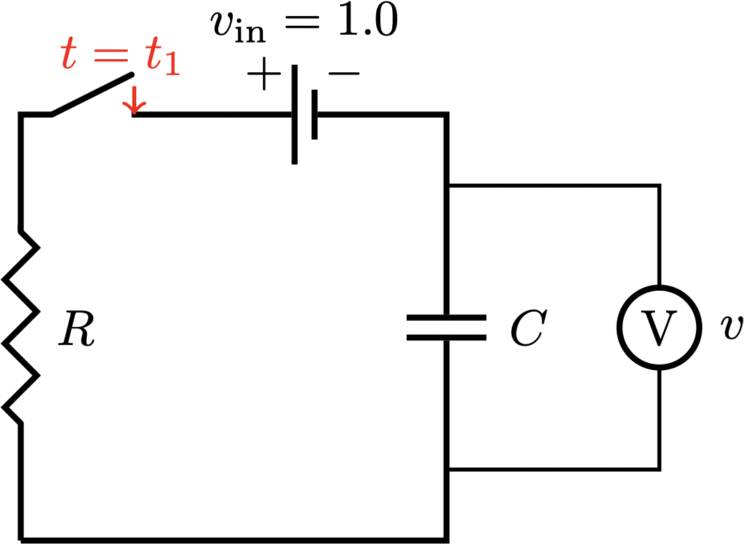
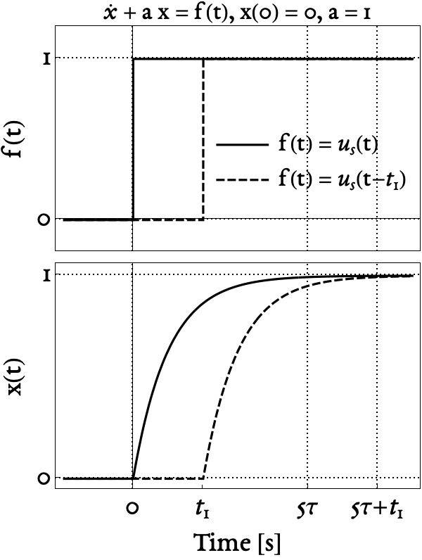
• What is the output of a first-order system if the input is the unit step function \(u_s(t)\) ? \[\dot{x} + ax = u_s(t) = \begin{cases} 1 & t > 0 \\ 0 & t < 0 \end{cases}, \quad x(0) = 0 \tag{1}\]
• Physically, this is equivalent to the following circuit:

• In-class task: What’s \(x(t)\) from Equation 1 ?

Step Response of First Order System

• The correct way to write the step response of a first-order system \(\dot{x} + ax = u_s(t)\) is \[ x(t) = \begin{cases} \displaystyle \frac{\left( 1- e^{-at} \right)}{a} & t > 0 \\ 0 & t < 0 \end{cases} \]

• This is equivalent to \[ x(t) = \displaystyle u_s(t) \frac{\left( 1- e^{-at} \right)}{a} \]

Step Response of Shifted First Order System

• What is the output of a first-order system if the input is the shifted unit step function \(u_s(t-t_1)\) ? \[\dot{x} + ax = u_s(t-t_1) = \begin{cases} 1 & t > t_1 \\ 0 & t < t_1 \end{cases}, \quad x(0) = 0 \tag{2}\]
• Physically, this is equivalent to the following circuit:

• In-class task: If \(x(t)\) for an un-shifted unit step input is \(\displaystyle \begin{cases} \displaystyle \frac{\left( 1- e^{-at} \right)}{a} & t > 0 \\ 0 & t < 0 \end{cases}\), what’s \(x(t)\) from Equation 2 ?

Shifted Step Response of First Order System

• The correct way to write the shifted unit step response of a first-order system \(\dot{x} + ax = u_s(t-t_1)\) is \[ x(t) = \begin{cases} \displaystyle \frac{\left( 1- e^{-a(t-t_1)} \right)}{a} & t > t_1 \\ 0 & t < t_1 \end{cases} \]

• This is equivalent to \[ x(t) = \displaystyle u_s(t-t_1) \frac{\left( 1- e^{-a(t-t_1)} \right)}{a} \]

Summarizing the step response and shifted step response

Step Response: \[ x(t) = \displaystyle u_s(t) \frac{\left( 1- e^{-at} \right)}{a} \]

Shifted Step Response: \[ x(t) = \displaystyle u_s(t-t_1) \frac{\left( 1- e^{-a(t-t_1)} \right)}{a} \]

Putting these together to get pulse response

• The output when the input is a step function, a.k.a. the step response, is a building block for pulse response.
• Approach: ‘piece together the answer’ (valid but tricky)
• Use Laplace Transform and the time-shifting property

The time-shifting property and Laplace Transforms

\[ \begin{aligned} \mathcal{L}\left[ f(t-D) \cdot u_s(t-D) \right] &= e^{-sD} F(s) \\ \mathcal{L}^{-1}\left[ e^{-sD} F(s) \right] &= f(t-D) \cdot u_s(t-D) \end{aligned} \]

• The Laplace Transform of a function shifted forward in time by \(D\) seconds equals to the Laplace Transform of that function (unshifted), multiplied by \(e^{-sD}\)
• In general, the functions should be zero for \(t < 0\) before you shift them!

The pulse response

\[\dot{x} + 2 x = 3 u_s(t) - 3 u_s(t-2.5)\] Solve for \(x(t)\) when \(f(t)\) is as shown to the left, i.e., a pulse of height \(3\) and duration \(2.5\)

In-class task: Find solution with one step function as input

• First, we approach \(\dot{x} + 2 x = 3 u_s(t)\)
• Applying Laplace Transforms, we get \[ sX(s) + 2 X(s) = \frac{3}{s} \implies X(s) = \frac{3}{s(s+2)} \]
• Which can be broken up into partial fractions \[ \frac{3}{2} \frac{1}{s} - \frac{3}{2} \frac{1}{s+2} \]
• And then re-converted into the sum of two terms in the time domain:

1. \(\displaystyle \frac{3}{2} u_s(t)\), a unit step function multiplied by a constant, and
2. \(\displaystyle - \frac{3}{2} e^{-2t}\), when \(t > 0\)

• So the result is \[ x(t) = \begin{cases} \displaystyle \frac{3}{2} \left( 1 - e^{-2t} \right) & t > 0 \\ 0 & t < 0 \end{cases} \]

In-class task: Find solution with the other step function as input

• Next, we approach \(\dot{x} + 2 x = -3 u_s(t-2.5)\)

• Applying Laplace Transforms, we get \[ sX(s) + 2 X(s) = -\frac{3}{s}e^{-2.5s} \implies X(s) = \frac{1}{s+2} \frac{-3}{s} e^{-2.5s} \]

• Which can be broken up into partial fractions \[ -\frac{3}{2} \frac{1}{s} e^{-2.5s} + \frac{3}{2} \frac{1}{s+2} e^{-2.5s} \]

• Each of these can be brought back into the time domain by shifting some function to the right by \(2.5\) seconds. \[ \underbrace{-\frac{3}{2} \frac{1}{s}}_{\text{Shift this}} e^{-2.5s} + \underbrace{\frac{3}{2} \frac{1}{s+2}}_{\text{Shift this}} e^{-2.5s} \]

• We read the highlighted terms off the table and find \[ \begin{aligned} \mathcal{L}^{-1} \left[ -\frac{3}{2} \frac{1}{s} \right] &= -\frac{3}{2} u_s(t) \\ \mathcal{L}^{-1} \left[ \frac{3}{2} \frac{1}{s+2} \right] &= \frac{3}{2} e^{-2t} \quad \text{when } t > 0 \end{aligned} \]

• Then we shift the result to the right, term by term: \[ x(t) = {-\frac{3}{2} u_s(t-2.5)} + {\frac{3}{2} e^{-2(t-2.5)} u_s(t-2.5)} \]

• We now have the response of the system to the other step function.

• So the result is \[ x(t) = -\frac{3}{2} u_s \left(t-5/2 \right) + \frac{3}{2} u_s \left( t-5/2 \right ) e^{-2(t-5/2)} \]

Putting it together

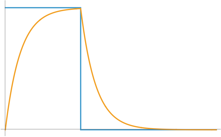
A note about the length of a pulse

• Depending on the duration of a pulse, the output of the system may look very different.

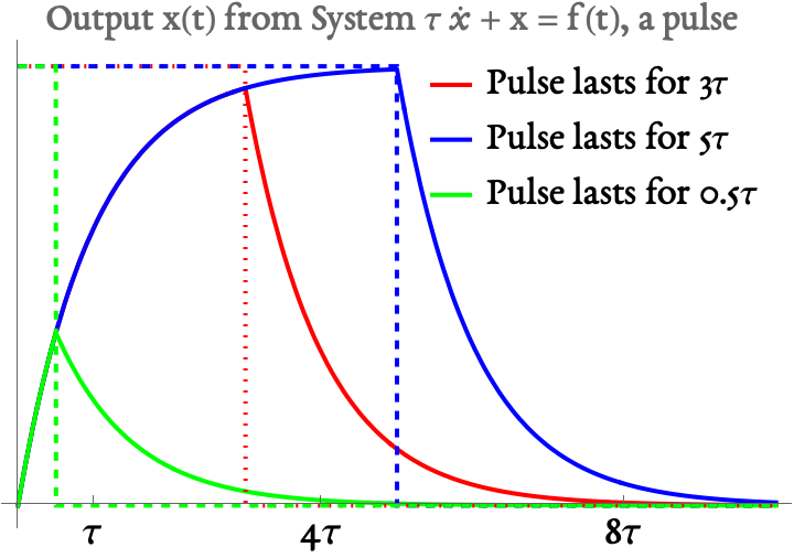
• What matters is how the duration compares with \(\tau\)

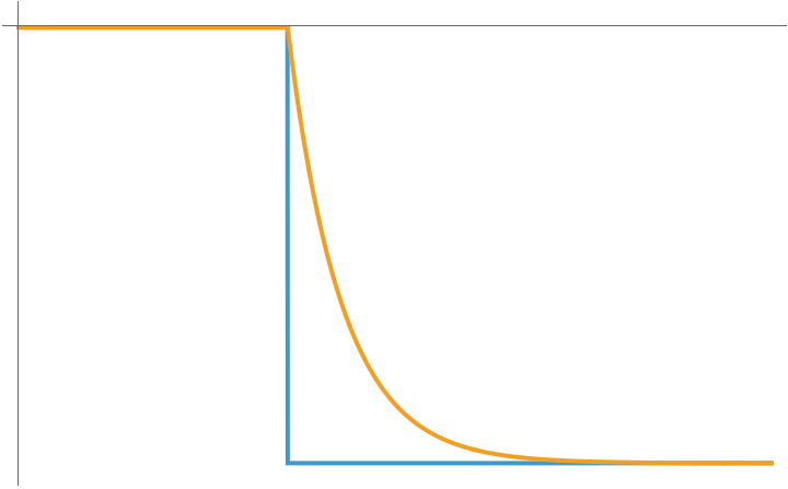
Response of a First-order system to \(\delta(t)\) input

• \(\delta(t)\) is also known as the ‘unit impulse’ function, or the Dirac Delta function.
• \(\delta(t)\) is the derivative of the unit step function, i.e.

The unit impulse response of a system equals the time-derivative of the (unit) step response

Consider the system \(\dot{x} + a x = f(t)\) where the input is \(f(t)\).

• If the input is a step, \(f(t) = u_s(t)\) the output is called the step response: \[x(t) = \begin{cases} \displaystyle \frac{1 - e^{-at}}{a} & t > 0 \\ 0 & t < 0 \end{cases}\]

• To obtain \(x(t)\) when the input is an impulse, \(f(t) = \delta(t)\),

• differentiate the unit step response w.r.t time: \[x(t) = \begin{cases} \displaystyle e^{-a t} & t > 0 \\ 0 & t < 0 \end{cases}\] which is known as the impulse response

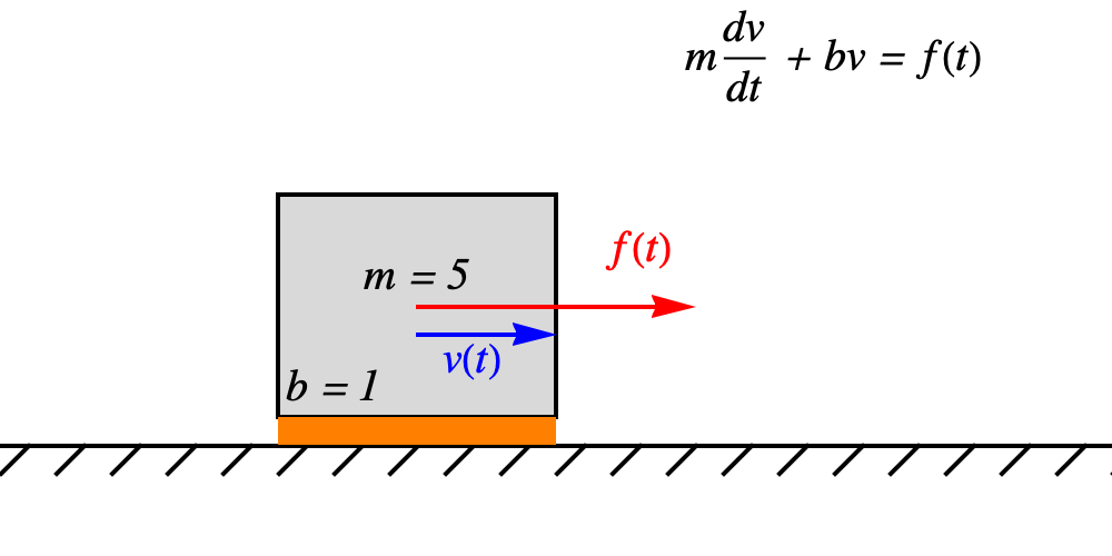
In-class task: What is the impulse response of the system below in terms of \(m\) and \(b\)?

Shifted Impulse Response

• The impulse need not be located at \(t=0\).
• We can easily move the impulse response to a later time.

Response of the system to a unit impulse applied at \(t = 0\):

\[ x(t) = \begin{cases} \displaystyle \frac{1}{m}e^{-t b / m} & t > 0 \\ 0 & t < 0 \end{cases} \]

Response of the system to a unit impulse applied at \(t = t_1\):

\[ x(t) = \begin{cases} \displaystyle \frac{1}{m}e^{-(t- t_1) b / m} & t > t_1 \\ 0 & t < t_1 \end{cases} \]

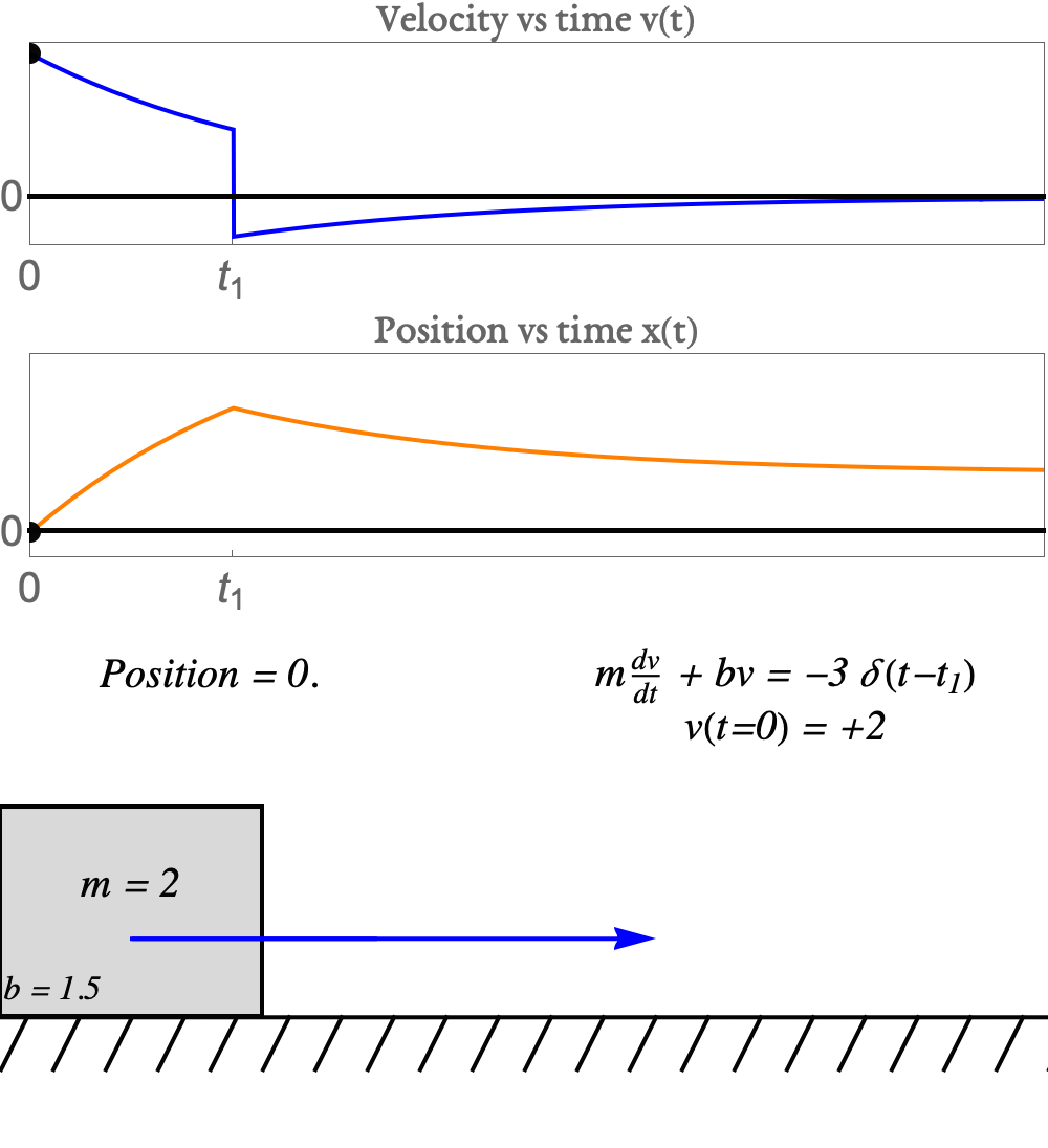
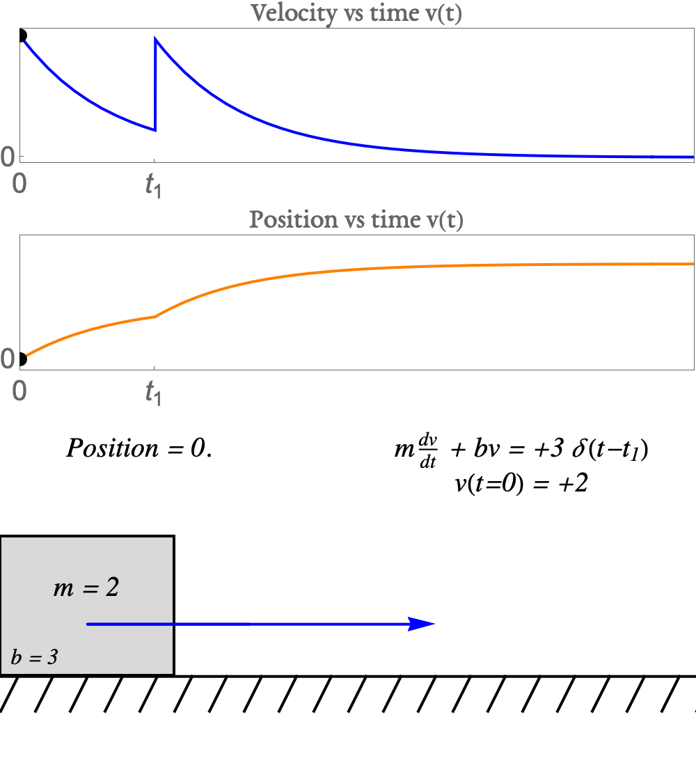
Using a shifted impulse function to represent impact

• Consider the model \[m \dot{x} + b x = f(t), \quad v(0) = v_0 \neq 0\]

• Let the force experienced by the object be a whack at a time \(t_1 > 0\).

• Then, we can use the input \(f(t) = A \delta(t-t_1)\) where \(A\) is the area under the force-time curve.

But what is an impulse?

• Recall Newton’s 2nd Law \(m\dot{v} = f\)
• What if the force is applied over a period of time?
• Integrate! from \(t_1\) to \(t_2\), we get \[m v_2 - m v_1 = \int_{t_1}^{t_2} f(t) dt\]
• Impulse: The change in momentum of an object, i.e., \(\int f dt\)
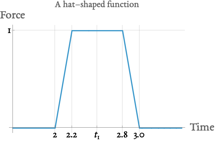
• A sudden change at \(t = t_1\) can be modeled by any of the following forces. (Thinner the ‘better’!)

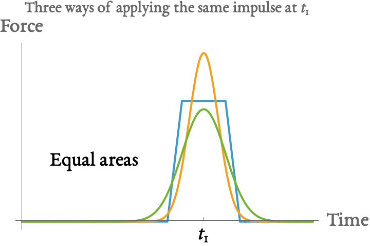
• Same quantity of impulse, applied in different ways; response slightly different
• Idealized impulse is \(\delta(t)\) (often called just ‘impulse’ or ‘unit impulse’)

The Shifted Ramp function and its uses

• A shifted ramp function with slope \(c\) and delay \(D\) can be constructed like: \[f(t) = \begin{cases} u_s(t - D) c(t - D) & t > D \\ 0 & t < D \end{cases}\]

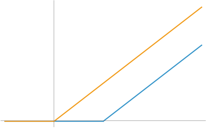
Using shifted ramp functions

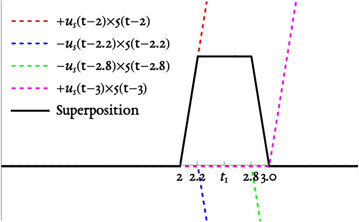
In-class task: Write down a formula for the following function using superposition of 4 (shifted and scaled) ramp functions

\[f(t) = \begin{cases} u_s(t - D) c(t - D) & t > D \\ 0 & t < D \end{cases}\]

The Transfer Function of a system and the Impulse Response of that system

Consider the system \[m \dot{v} + b v = f_a(t)\] where \(v(t)\) is the output and \(f_a(t)\) the input.

Find the transfer function

\[ \begin{aligned} m s V(s) + b V(s) = F_a(s)& \\ V(s) = \frac{1}{ms + b} F_a(s)& \\ \implies \frac{V(s)}{F_a(s)} = \underbrace{\boxed{\frac{1}{m s + b}}}_{\text{Transfer Function}}& \end{aligned} \]

Find \(v(t)\) when \(f_a(t) = \delta (t)\)

\[ \begin{aligned} m s V(s) + b V(s) &= \mathcal{L} \left[ \delta (t) \right] \\ m s V + b V &= 1 \\ \implies V(s) = \underbrace{\boxed{\frac{1}{ms+b}}}_{\text{Impulse Response}} \end{aligned} \]

Tip

The Transfer Function of a system is also the Laplace Transform of that system’s (unit) impulse response.