For a linear differential equation, the sum of two solutions is also a solution.
For a linear differential equation, a constant times a solution is also a solution.
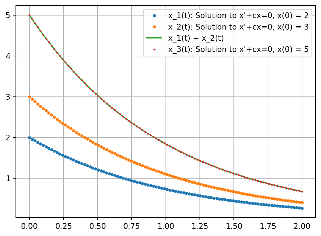
Illustrating linearity
An RC circuit in which the capacitor is initially at 2 Volts.
An RC circuit in which the capacitor is initially at 3 Volts.
\[RC \dot{v} + v = 0, \qquad v(0) = 2 \text{ or } 3 \]
\(v(0) = 2\)
Solution: \(v(t) = 2 e^{-t}\)
\(v(0) = 3\)
Solution: \(v(t) = 3 e^{-t}\)
Can we use solutions to these to predict what happens if \(v(0) = 5\)?
Superposition of two solutions
Code
import numpy as npfrom scipy.integrate import solve_ivpimport matplotlib.pyplot as pltRC =1V0 =3# Set up time domaint_f =2t_vals = np.linspace(0,t_f,100)def V_sum(t):return5*np.exp(-1/(RC)*t)def ode_rhs(t,X):return (-1/RC)*X[0]sol1_ode = solve_ivp(ode_rhs, [0,t_f],[2],t_eval=t_vals)sol2_ode = solve_ivp(ode_rhs, [0,t_f],[3],t_eval=t_vals)sol3_ode = solve_ivp(ode_rhs, [0,t_f],[5],t_eval=t_vals)plt.plot(t_vals, sol1_ode.y[0],'.',label="x_1(t): Solution to x'+cx=0, x(0) = 2")plt.plot(t_vals, sol2_ode.y[0],'.',label="x_2(t): Solution to x'+cx=0, x(0) = 3")plt.plot(t_vals, sol1_ode.y[0]+sol2_ode.y[0],'-',label="x_1(t) + x_2(t)")plt.plot(t_vals, sol3_ode.y[0],'.',label="x_3(t): Solution to x'+cx=0, x(0) = 5",markersize=3)plt.legend()plt.grid()plt.show()
Steady State
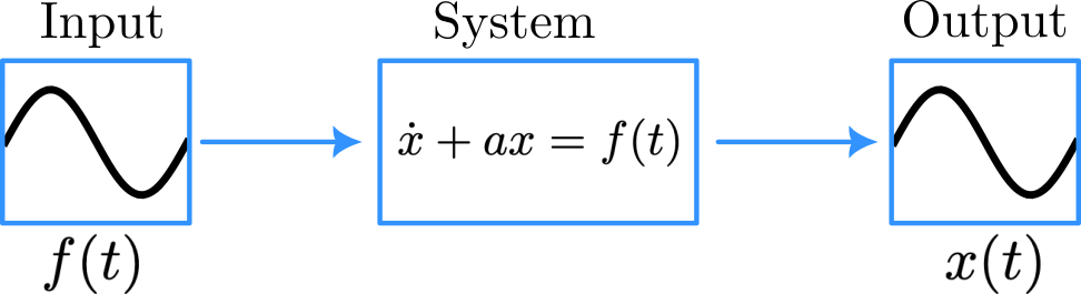
\[\dot{x} + a x = f(t) \]
If we call \(f(t)\) the ‘input’ and \(x(t)\) the ‘response’, then:
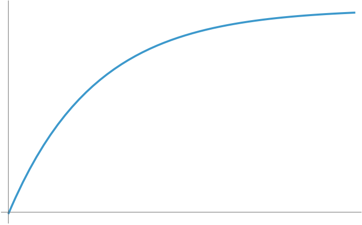
\(x(t)\) eventually reaches a steady state, i.e., \(x(t)\) settles into some long-term behavior that depends on \(f(t)\).
The steady-state behavior of \(x(t)\) can be
zero,
or a constant,
or some other function of time, depending on \(f(t)\).
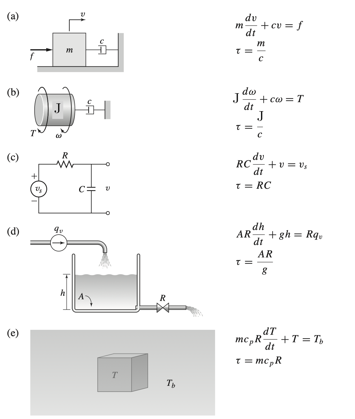
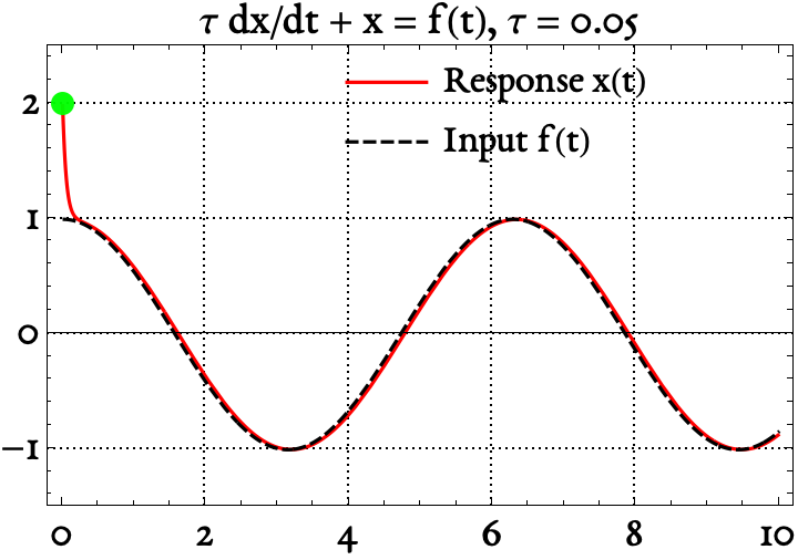
A ‘time scale’ for first-order systems
Consider the first-order system \(RC \dot{v} + v = f(t)\)
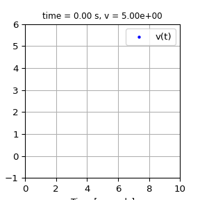
If \(f(t) = 0\) and \(v(0) = 5\), the solution is
Code
import numpy as npimport matplotlib.pyplot as pltimport matplotlib.animation as animationfig, ax = plt.subplots()N =100t_end =10t = np.linspace(0, t_end, N)def ft(t):return5*np.exp(-t)v = ft(t)fig.set_figwidth(3.0)fig.set_figheight(3.0)scat = ax.scatter(t[0], v[0], c="b", s=5, label='v(t)')ax.set(xlim=[0, t_end], ylim=[-1, 6])ax.set_xlabel('Time [seconds]',fontsize=9)ax.set_ylabel('V [volts]', fontsize=9)plt.grid()ax.legend()def update(frame):# for each frame, update the data stored on each artist. x = t[:frame] y = v[:frame]# update the scatter plot: data = np.stack([x, y]).T scat.set_offsets(data) ax.set_title(f'time = {t[frame]:.2f} s, v = {v[frame]:.2e}',fontsize=9) return scatani = animation.FuncAnimation(fig=fig, func=update, frames=N, interval=30)writer1 = animation.PillowWriter(fps=15) # Set frames per second (fps)ani.save("first-order.gif",writer = writer1)
When should we say the system has decayed ‘completely’?
Never truly reaches zero
We need a ‘time scale’ to talk about
‘how quickly this system decays’
‘when the system has decayed completely’
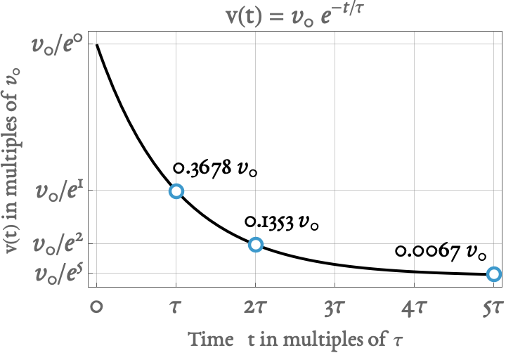
The time constant \(\tau\)
We found that the first-order system \(RC \dot{v} + v = 0\) with initial condition \(v(0) = v_0\) has solution \[v(t) = v_0 e^{-\frac{t}{RC}}\]
Let’s now define a new parameter \(\tau = RC\) called the time constant such that \[v(t) = v_0 e^{-\frac{t}{\tau}}\]
What are the units of \(\tau\)?
TipThe time constant \(\tau\) is measured in seconds.
Mathematically speaking, the function \(e^x\) applies to pure numbers \(x\). So \(t\) and \(\tau\) must have the same units. Thus, \(\tau\) is measured in seconds or multiples of it.
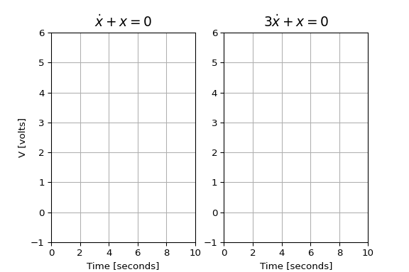
Every first-order linear system has a time constant
The time constnat \(\tau\)
measures how long a first-order system takes to settle down to a steady-state value
Code
import numpy as npimport matplotlib.pyplot as pltimport matplotlib.animation as animationfig, ax = plt.subplots(ncols=2)N =100t_end =10t = np.linspace(0, t_end, N)tau =3def ft(t):return5*np.exp(-t)def ft2(t):return5*np.exp(-t/tau)v = ft(t)v2 = ft2(t)fig.set_figwidth(6)fig.set_figheight(4)scat1 = ax[0].scatter(t[0], v[0], c="b", s=5)ax[0].set(xlim=[0, t_end], ylim=[-1, 6])ax[0].set_xlabel('Time [seconds]',fontsize=10)ax[0].set_ylabel('V [volts]', fontsize=10)scat2 = ax[1].scatter(t[0], v[0], c="b", s=5)ax[1].set(xlim=[0, t_end], ylim=[-1, 6])ax[1].set_xlabel('Time [seconds]',fontsize=10)ax[0].grid(True)ax[1].grid(True)ax[0].set_title(r"$\dot{x} + x = 0$",fontsize=14)ax[1].set_title(r"$3\dot{x} + x = 0$",fontsize=14)def update(frame):# for each frame, update the data stored on each artist. x = t[:frame] y = v[:frame]# also for the other plot y2 = v2[:frame]# update the scatter plot: data = np.stack([x, y]).T scat1.set_offsets(data) scat2.set_offsets(np.stack([x,y2]).T)# ax[0].set_title(f'time = {t[frame]:.2f} s, v = {v[frame]:.2e}',fontsize=9) # ax[1].set_title(f'time = {t[frame]:.2f} s, v = {v2[frame]:.2e}',fontsize=9) return (scat1,scat2)ani = animation.FuncAnimation(fig=fig, func=update, frames=N, interval=30)writer1 = animation.PillowWriter(fps=10) # Set frames per second (fps)# plt.show()ani.save("timeconst-comparison.gif",writer = writer1)
The time constant \(\tau\)
provides convenient sign-posts to talk about how far a system is from reaching ‘steady-state’
When \(t = 1\tau\), the response is 63.3% of the way toward reaching steady-state
When \(t = 2\tau\), the response is 86.5% of the way toward reaching steady-state
When \(t = 5\tau\), the response is 99.4% of the way toward reaching steady-state.
Time
Value
Decimal
Percent
\(t=0 \tau\)
\(v=v_0 e^{-0}\)
\(v=1.0 v_0\)
100%
\(t=1 \tau\)
\(v=v_0 e^{-1}\)
\(v=0.3678v_0\)
36.7%
\(t=2 \tau\)
\(v=v_0 e^{-2}\)
\(v=0.1353 v_0\)
13.5%
\(t=3 \tau\)
\(v=v_0 e^{-3}\)
\(v=0.0497 v_0\)
4.9%
\(t=4 \tau\)
\(v=v_0 e^{-4}\)
\(v=0.0183 v_0\)
1.8%
\(t=5 \tau\)
\(v=v_0 e^{-4}\)
\(v=0.0067 v_0\)
0.6%
At what value of time is \(v(t)\) equal to half its initial value? Give your answer in multiples of \(\tau\).
At what value of time is \(v(t)\) equal to 0.1 percent of its original value?
In-class design example
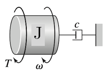
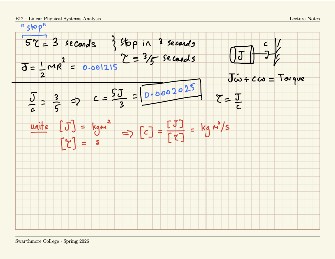
A motor shaft continues to spin after the motor is switched off, slowly slowing down due to friction. No more external power is provided to the shaft during this motion. At the moment it’s switched off, it has a rotational speed of 1200 RPM.
For a shaft, \(J = \frac{1}{2}m r^2\).
Mass = 2.7 kg and radius = 3.0 cm.
Design requirement
Shaft must spin down to a stop in 3 seconds.
Radians should be considered unitless
Calculate how much \(c\) should be to meet the design requirement.
What are the units of \(c\) in SI?
TipGoverning equation
\[
J \frac{d \omega}{dt} + c \omega = T
\]
\(T\): Torque \(\omega\): Angular velocity \(c\): Amount of (dynamic) friction
Steady-state response for first-order systems
Let’s consider 4 types of input:
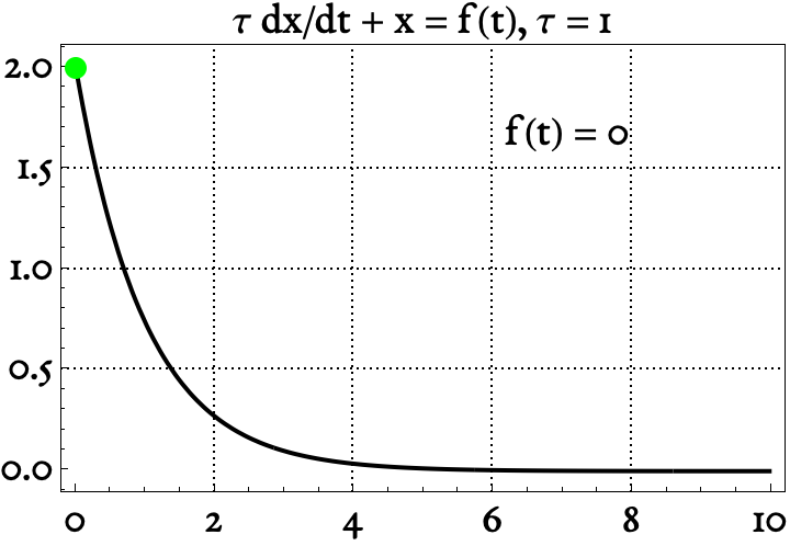
\(f(t) = 0\)
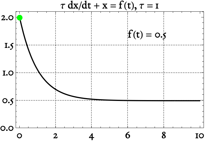
\(f(t) = \text{const.}\)
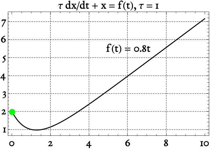
\(f(t) = c t\)
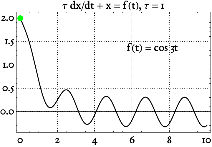
\(f(t) = \cos(\omega t)\)
(lab 1) \(f(t) =\) an impulse
Transient vs. steady-state
\[\dot{x} + ax = f(t)\]
Input
Transient Response
Steady-State Response
\(f(t) = 0\)
\(x_0 e^{-at}\)
\(0\)
\(f(t) = k\)
\(e^{-at} \left( x_0 -k \right)\)
\(k\)
\(f(t) = c t\)
\(f(t) = \cos \omega t\)
\(f(t) =\) impulse (lab 1)
First-order Response to zero input
First-order Response to constant input
First-order Response to ramp input
First-order Response to periodic input
Response of first-order systems
Input
Response
\(f(t) = 0\)
\(f(t) = k\)
\(f(t) = c t\)
\(f(t) = \cos \omega t\)
Transient and steady-state
Transient and steady-state components of a solution \(x(t)\) can be mathematically defined
Approximately, we can say that steady-state sets in after \(5\tau\) units of time have passed.
Numerical Solution of differential equations
When \(\dot{x} = f(x,t)\) is too hard to integrate symbolically, we can use a computer.
Analytical
Numerical
is written mathematically as \(x(t) =\) some function of time.
is stored in a computer as a series of points \((t_k, x_k)\)
Once analytical solution is known, you can calculate \(x\) for any \(t\) you want.
interpolation must be used between calculated points
Accurate and as precise as can be
Usually accurate and ‘precise enough’
Only wrong if you make an algebra mistake
Can be wrong even if there are no algebra mistakes and eqaution is correctly entered into computer program
functiondxdt=rhs1(t,x)% return the value of f(x,t)dxdt=t-x;end% Time span over which to integratetspan=linspace(0,6,30);x0=3;% Call ode45 and assign solution to x.[t,x] =ode45(@rhs1,tspan,x0);% Plotplot(t,x,'o-')
1
The right hand side of \(\dot{x} = f(x,t)\)
2
Integrate from \(t=0\) to \(t=6\) and calculate at 30 points
3
Initial condition
4
Syntax for ode45.
numerical_solution.py
import numpy as npimport matplotlib.pyplot as pltfrom scipy.integrate import solve_ivpdef rhs1(t,x):# return the value of f(x,t)return t - x[0]# Time span over which to integratetspan = np.linspace(0,6,30) x0 = [3]sol = solve_ivp(rhs1,tspan[[0,-1]],x0,t_eval=tspan)# Plot the solutionplt.plot(sol.t,sol.y[0],'o-'); plt.show()
1
Packages must be imported
2
The right hand side of \(\dot{x} = f(x,t)\)
3
Initial condition has to be given as a list or array
4
Provide start/end points and t_eval=
5
Plot using attributes t and y of object of type OdeResult returned by solve_ivp.
sol =NDSolve[{x'[t]+x[t]==t,x[0]==3},x[t],{t,0,6}]Plot[x[t]/. sol,{t,0,6}]