For a differential equation of order \(n\), you need \(n\) initial conditions to have a ‘well-posed Initial Value Problem’
First-order IVP \[
\begin{align}
\dot{x} &= f(x,t) \\
x(0) &= \text{ some value }
\end{align}
\]
Second-order IVP \[
\begin{align}
\ddot{x} &= f(x,\dot{x},t) \\
x(0) &= \text{ some value } \\
\dot{x}(0) &= \text{ some other value }
\end{align}
\]
Note about class progression
Week
Lecture Topic
Due
Lab
1
Math preliminaries
HW 0
2
First-order systems in time domain
HW 1
1: Impulse Response
3
Frequency domain; Laplace Transform
HW 2
1: Impulse Response
4
Block diagrams & Simulink
HW 3
2: Numerical Soln
5
Second-order systems with no damping
HW 4
2: Numerical Soln
6
State-variable approach
HW 5
3: Biomechanics
7
Second-order systems with damping
HW 6
3: Biomechanics
8
Mechanical modeling of coupled sys
Midterm 03/19 7PM
4: Coupled pendulum
9
Damping ratio, settling time, etc.
HW 7
No Lab
10
Second-order systems with Laplace
HW 8
4: Coupled pendulum
11
Bode plots
HW 9
No Lab
12
Introduction to Fourier Series
HW 10
5: Fourier Series
13
Vibrations; modes; normal modes
HW 11
5: Fourier Series
14
Further second-order models
HW 12
A simple second-order differential equation
Consider the differential equation \[
\ddot{y} = -g
\]
with two initial conditions \[
\begin{align}
\dot{y} &= 5 \text{ at } t = 0 \\
y &= 3 \text{ at } t = 0
\end{align}
\]
To solve this, let’s write it as \[
\frac{d}{dt} \frac{dy}{dt} = -g
\]
Multiplying by \(dt\) and integrating once, we get \[
\int d \left( \frac{dy}{dt} \right) = \int -g dt
\]
Which simplifies to \[
\frac{dy}{dt} = \dot{y} = -g \cdot t + c_1
\]
We can now use our first initial condition “\(\dot{y} = 5\) when \(t = 0\)” to solve for \(c_1\): \[
5 = -g \cdot 0 + c_1 \implies c_1 = 5 \implies \dot{y} = -gt + 5
\]
Now, we integrate again \[
\begin{align}
\dot{y} = \frac{dy}{dt} &= -gt + 5 \\
\int dy &= \int (- gt + 5) dt
\end{align}
\]
and by the usual rules of integration, we find \[
\begin{align}
y &= -\frac{1}{2} g t^2 + 5t + c_2 \\
\end{align}
\]
Now, we use our second initial condition “\(y = 3\) when \(t = 0\)” to solve for \(c_2\). \[
3 = -\frac{1}{2} g (0)^2 + 5(0) + c_2 \implies c_2 = 3
\]
So the solution to our initial value problem is \[
\boxed{y(t) = -\frac{1}{2} g t^2 + 5t + 3}
\]
Back to first-order systems
In this class, we are concerned with systems of the kind \[
\dot{x} = f(x,t)
\] where \(f\) is linear in \(x\).
We can write all linear first-order systems in the form \[
\boxed{\dot{x} + a x= f(t)}
\] where \(f\) is a different function; now only a function of time.
\(a\) is a constant. Does not depend on \(x\) or \(t\).
Often, but not always:
\(x(t)\) is the output: what you want to know about
and \(f(t)\) is the input: what you control
First-order systems: types of input
We will tackle first-order systems \[\dot{x} + a x = f(t)\] in order of increasing complexity of \(f(t)\)
\(f(t) = 0\) (‘unforced’ system)
\(f(t) = \text{const.}\) (‘constant input’)
\(f(t) = c t\) (‘ramp input’)
\(f(t) = \sin(\omega t)\) (‘periodic input’)
\(f(t) =\) ‘arbitrary input’
Integrating gets more difficult
Introduce other tools including Laplace Transform, ode45/solve_ivp
An example first-order system from E11
A voltage source \(v_i(t)\) is applied
Voltage is measured using perfect voltmeters at both \(C_1\) and \(R_1\).
Start with \(v_i(t) = 0\)
In this case, \(v_C = v_R = v\).
An example first-order system from E11
Resistor \(\displaystyle i_R = \frac{v}{R}\)
Capacitor: \(\displaystyle i_C = C \frac{d v}{dt}\)
Note that \(R\) and \(C\) are both always positive. \[R C \frac{dv}{dt} + v = 0 \]
Solving first-order RC circuits with no input
\[RC \frac{dv}{dt} + v = 0\]
\[ \frac{dv}{dt} + \frac{1}{RC} v = 0\]
Suppose we start with \(v(0) = 5\) volts across the capacitor.
To solve this system, rearrange and integrate \[
\int dv = - \int (1/RC) v dt
\]
which is straightforward \[
\begin{align}
\int \frac{dv}{v} &= - \int (1/RC) dt \\
\implies \log v &= - \frac{t}{RC} + c_1 \\
\implies e^{\log v} &= e^{ -\frac{t}{RC} + c_1} = e^{-\frac{t}{RC}} e^{c_1} \\
\implies v &= ke^{-\frac{t}{RC}}
\end{align}
\]
Then, we use the initial condition \[
5 = k e^{0} \implies k = 5
\]
to write down the particular solution \[
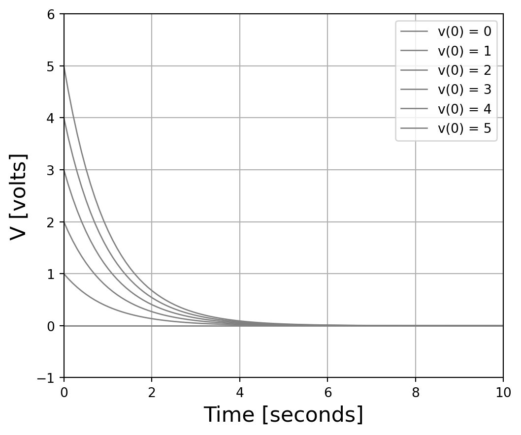
\boxed{v(t) = 5e^{-\frac{t}{RC}}}
\]
now, let’s plot it assuming \(RC=1\).
Illustrating first-order systems
Code
import numpy as npimport matplotlib.pyplot as pltimport matplotlib.animation as animationfig, ax = plt.subplots()N =100t_end =10t = np.linspace(0, t_end, N)def ft(t):return5*np.exp(-t)v = ft(t)scat = ax.scatter(t[0], v[0], c="b", s=5, label='v(t)')ax.set(xlim=[0, t_end], ylim=[-1, 6])ax.set_xlabel('Time [seconds]',fontsize=16)ax.set_ylabel('V [volts]', fontsize=16)plt.grid()ax.legend()def update(frame):# for each frame, update the data stored on each artist. x = t[:frame] y = v[:frame]# update the scatter plot: data = np.stack([x, y]).T scat.set_offsets(data) ax.set_title(f'time = {t[frame]:.2f} s, v = {v[frame]:.2e}',fontsize=16) return scatani = animation.FuncAnimation(fig=fig, func=update, frames=N, interval=30)writer1 = animation.PillowWriter(fps=15) # Set frames per second (fps)ani.save("first-order.gif",writer = writer1)
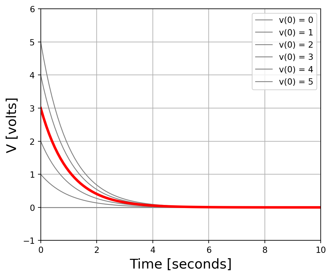
A first-order RC circuit \(RC \dot{v} + v = 0\)
Code
import numpy as npimport matplotlib.pyplot as pltimport matplotlib.animation as animationfig, ax = plt.subplots()N =100t_end =10t = np.linspace(0, t_end, N)def ft(t,v0):return v0*np.exp(-t)v0s =list(range(6))vs = [ft(t,v0) for v0 in v0s]for j inrange(len(v0s)): plt.plot(t,vs[j],color="gray",linewidth=1,label="v(0) = "+str(v0s[j]))ax.set(xlim=[0, t_end], ylim=[-1, 6])ax.set_xlabel('Time [seconds]',fontsize=16)ax.set_ylabel('V [volts]', fontsize=16)ax.legend()plt.grid()fig.set_figwidth(6) plt.show()
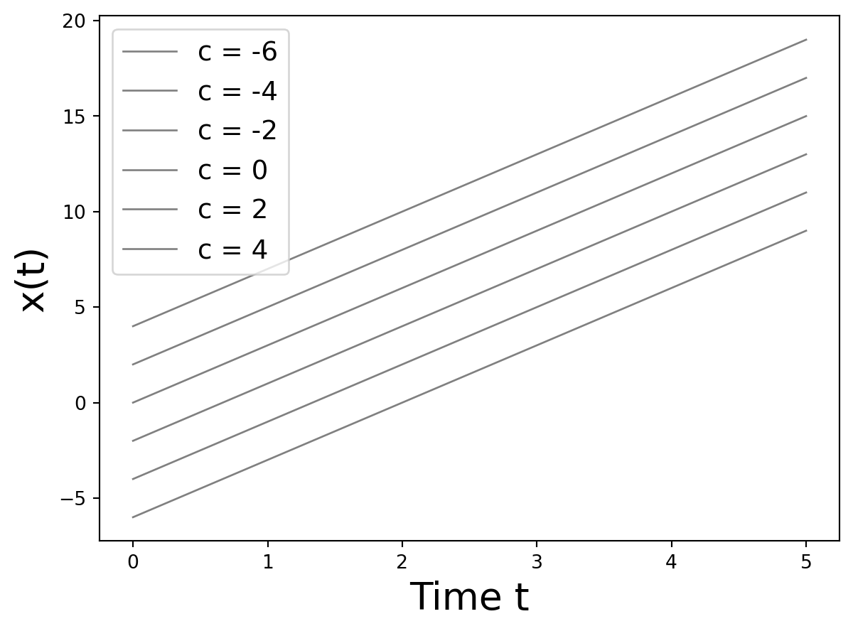
General solution \[v(t) = c e^{-t/RC}\] when initial condition is not specified
A first-order RC circuit \(RC \dot{v} + v = 0\)
Code
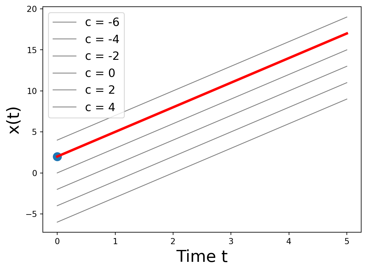
import numpy as npimport matplotlib.pyplot as pltimport matplotlib.animation as animationfig, ax = plt.subplots()N =100t_end =10t = np.linspace(0, t_end, N)def ft(t,v0):return v0*np.exp(-t)v0s =list(range(6))vs = [ft(t,v0) for v0 in v0s]for j inrange(len(v0s)): plt.plot(t,vs[j],color="gray",linewidth=1,label="v(0) = "+str(v0s[j]))ax.set(xlim=[0, t_end], ylim=[-1, 6])ax.set_xlabel('Time [seconds]',fontsize=16)ax.set_ylabel('V [volts]', fontsize=16)ax.legend()plt.grid()plt.plot(t,vs[3],linewidth=3,color="red")fig.set_figwidth(6) plt.show()
Particular solution \[\boxed{v(t) = 3 e^{-t/RC}}\] when initial condition is specified \(v(0) = 3\)
The mechanical/electrical analogy
Both systems have equations of the form \[\frac{dx}{dt} + (\text{some positive const.}) \times x = 0\]
\[RC \dot{v} + v = 0\]
\[m\dot{v} + bv = 0\]
and their solutions are decaying exponentials
A first-order system with an input
Recall that first order systems have the form \[
\dot{x} + a x = f(t)
\]
We looked at systems for which \(f(t) = 0\)
We will now consider the simplest \(f(t)\): a constant.
Electrical systems: D.C. current source or voltage source
Mechanical systems: constant force applied
An RC Circuit with constant voltage source
\(\displaystyle i_R = \frac{v_R}{R}\)
\(\displaystyle i_C = C\frac{d v_c}{dt}\)
use KCL and KVL to derive governing differential equation for \(v_C\)
An RC Circuit with constant voltage source
\(\displaystyle i_R = \frac{v_R}{R}\)
\(\displaystyle i_C = C\frac{d v_c}{dt}\)
use KCL and KVL to derive governing differential equation for \(v_C\)
The governing equation simplifies to \[
\boxed{RC \frac{d v_C}{dt} + v_C = v_s}
\]
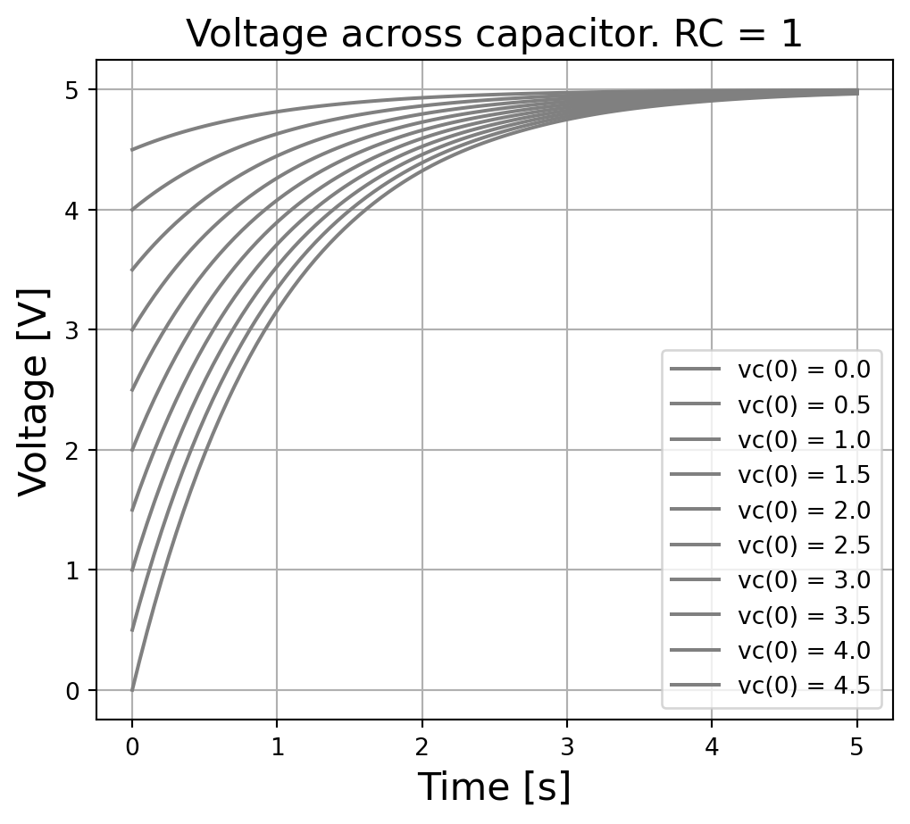
A first-order RC circuit \(RC \dot{v}_c + v_c = v_s\)
Let’s illustrate before we learn how to derive it
Code
import numpy as npimport matplotlib.pyplot as pltimport matplotlib.animation as animationfrom scipy.integrate import solve_ivpRC =1t_final =5N =100t_list = np.linspace(0,t_final,N)def rhs_diffeq(t,x):return (5- x)/RCinit_conds = np.arange(0,5,0.5)sol = solve_ivp(rhs_diffeq, [0,t_final], init_conds,t_eval=t_list)for j inrange(len(init_conds)): plt.plot(sol.t,sol.y[j],color='gray',label="vc(0) = "+str(init_conds[j]))plt.grid()plt.title("Voltage across capacitor. RC = 1",fontsize=16)plt.xlabel("Time [s]",fontsize=16)plt.ylabel("Voltage [V]",fontsize=16)plt.legend()plt.gcf().set_figwidth(6)plt.show()
General solution when initial condition is not specified
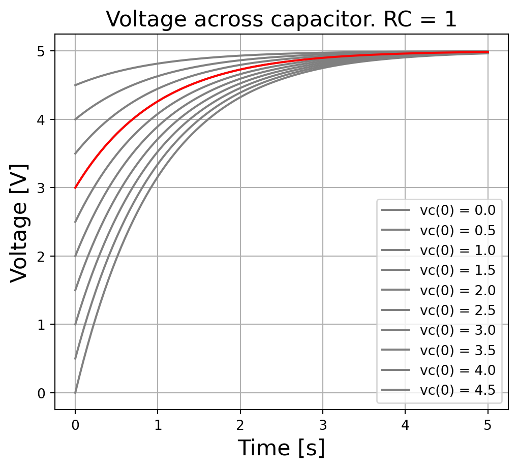
A first-order RC circuit \(RC \dot{v}_c + v_c = v_s\)
Let’s illustrate before we learn how to derive it
Code
import numpy as npimport matplotlib.pyplot as pltimport matplotlib.animation as animationfrom scipy.integrate import solve_ivpRC =1t_final =5N =100t_list = np.linspace(0,t_final,N)def rhs_diffeq(t,x):return (5- x)/RCinit_conds = np.arange(0,5,0.5)sol = solve_ivp(rhs_diffeq, [0,t_final], init_conds,t_eval=t_list)for j inrange(len(init_conds)): plt.plot(sol.t,sol.y[j],color='gray',label="vc(0) = "+str(init_conds[j]))plt.plot(sol.t,sol.y[6],color='red')plt.grid()plt.title("Voltage across capacitor. RC = 1",fontsize=16)plt.xlabel("Time [s]",fontsize=16)plt.ylabel("Voltage [V]",fontsize=16)plt.legend()plt.gcf().set_figwidth(6)plt.show()
Particular solution when initial condition is specified \(v_c(0) = 3\)
Solve \(RC \dot{v} + v = v_s\) with \(v(0) = v_0\)
Solve \(RC \dot{v} + v = v_s\) with \(v(0) = v_0\)
The solution is \[
\boxed{v(t) = \frac{3}{2} - \frac{3}{2} e^{-2t} + v_0 e^{-2t}} \qquad \qquad \qquad \qquad
\]
Solution viewed as transient plus steady-state terms: \[
v(t) = \underbrace{e^{-2t} \left[ v_0 - \frac{3}{2}\right]}_{\text{transient}} + \underbrace{\frac{3}{2}}_{\text{steady-state}}
\]
or as the sum of a forced response and a free response: \[
v(t) = \underbrace{\frac{3}{2}-\frac{3}{2}e^{-2t}}_{\text{forced response}} + \underbrace{v_0 e^{-2t}}_{\text{free response}}
\]
Note: This slide has been corrected on Jan 30
RC Circuit with ramp input
Recall: \[\dot{x} + a x = f(t) \]
\(f(t) = 0\) (‘unforced’ system) ✓
\(f(t) = \text{const.}\) (‘constant input’) ✓
\(f(t) = c t\) (‘ramp input’)
\(f(t) = \sin(\omega t)\) (‘periodic input’)
\(f(t) =\) ‘arbitrary input’
Variable voltage source is set to ‘ramp up’ \(v_s(t) = 3t\)
Equation is still \[RC \dot{v}_c + v_c = v_s\]
Solve \(RC \dot{v} + v = v_s(t)\) with \(v(0) = v_0\)
Let’s solve equation in this form: \[\frac{dx}{dt} + 2x = 3t\]
General solution is \[
\boxed{x(t) = ce^{-2t} + \frac{3}{2}t - \frac{3}{4}}
\] (We haven’t derived this yet)