Lecture 22
E12 Linear Physical Systems Analysis
April 9, 2026
Frequency Response of Second Order Systems
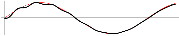
- Second-order systems subjected to a sinusoidal input, lead to a sinusoidal output once the transients have died out.
Frequency Response of Overdamped 2nd Order Systems
Recall that overdamped means \(\zeta > 1\) where \[\zeta = \frac{b}{2\sqrt{m k}}\]
An overdamped 2nd order system
\[ \begin{aligned} m &= 50 \\ b &= 100.5 \\ k &= 1 \end{aligned} \]
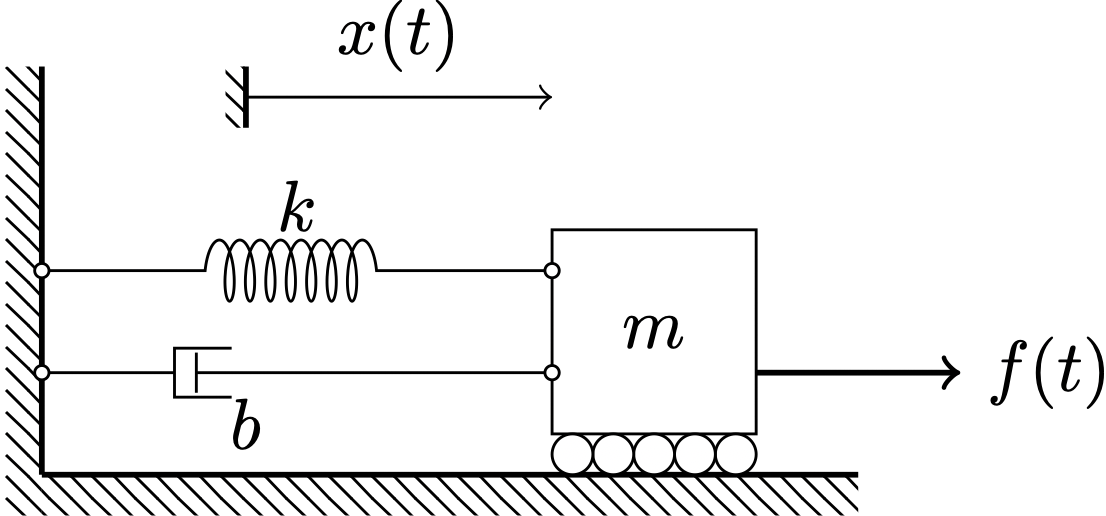
Differential equation of the system \[50 \ddot{x} + 100.5 \dot{x} + x = f(t)\]
Transfer function: \[T(s) = \frac{X(s)}{F(s)} = \frac{1}{50s^2 + 100.5s+1}\]
Using the roots of the denominator, we can re-write as \[T(s) = \frac{X(s)}{F(s)} = \frac{1}{(100s+1)(0.5s+1)}\]
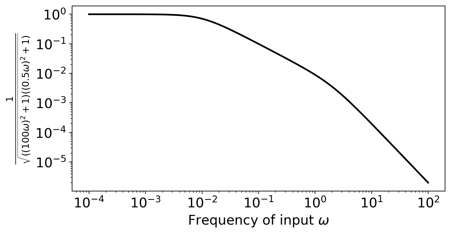
The (magnitude) Bode Plot needs the complex number \(\boxed{T(i\omega)}\) \[\left| T(i\omega) \right| = \left| \frac{1}{(100 i \omega +1)(0.5 i \omega + 1)}\right| = \frac{1}{\sqrt{\left( (100 \omega)^2 + 1 \right)\left( (0.5 \omega)^2 + 1 \right)}}\]
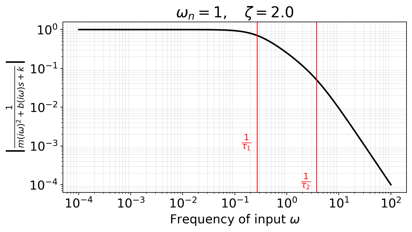
Bode Plot for overdamped 2nd order
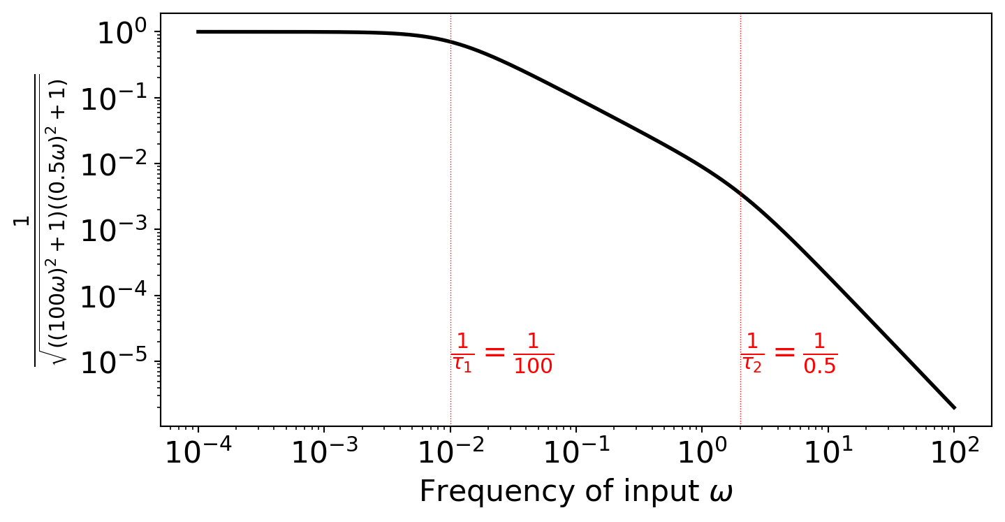
- When a second-order system is overdamped, \(m s^2 + b s + k\) has two real roots.
- Each root corresponds to a corner frequency.
- We often re-write, e.g., \(50 s^2 + 100.5s + 1\) as \((\tau_1 s + 1)(\tau_2 s +1)\)
Procedure for determining \(\tau_1\) and \(\tau_2\) for overdamped systems
Suppose \(m = 2, b = 14, k = 20\). Recall that \(\zeta = \frac{b}{2\sqrt{m k}}\).
Is this system overdamped? Yes! \(\zeta = \frac{14}{2 \sqrt{2 \times 20}} \approx 1.1\)
Given the diff. eq. \(\quad 2 \ddot{x} + 14 \dot{x} + 20 x = f(t), \quad\) write the transfer function for this system in the form \(\frac{...}{(\tau_1 s + 1)(\tau_2 s + 1)}\)
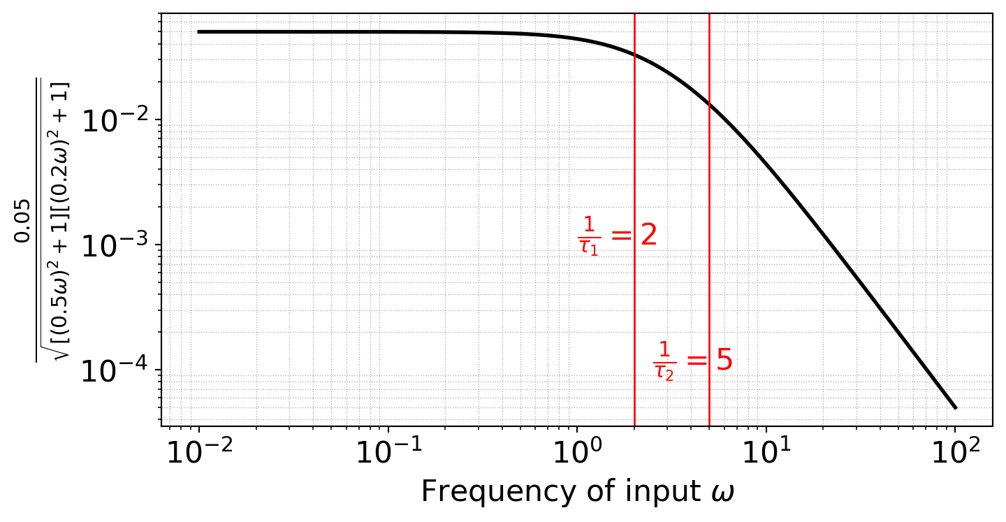
\(T(s) = \frac{X}{F} = \frac{1}{2 s^2 + 14s +20}\) \(= \frac{1}{2(s+2)(s+5)}\) \(= \frac{0.05}{(0.5s+1)(0.2s+1)}\)
So the corner frequencies of this system are \(1/\tau_1 = 1/0.5 = 2\) and \(1/\tau_2 = 1/0.2 = 5\)
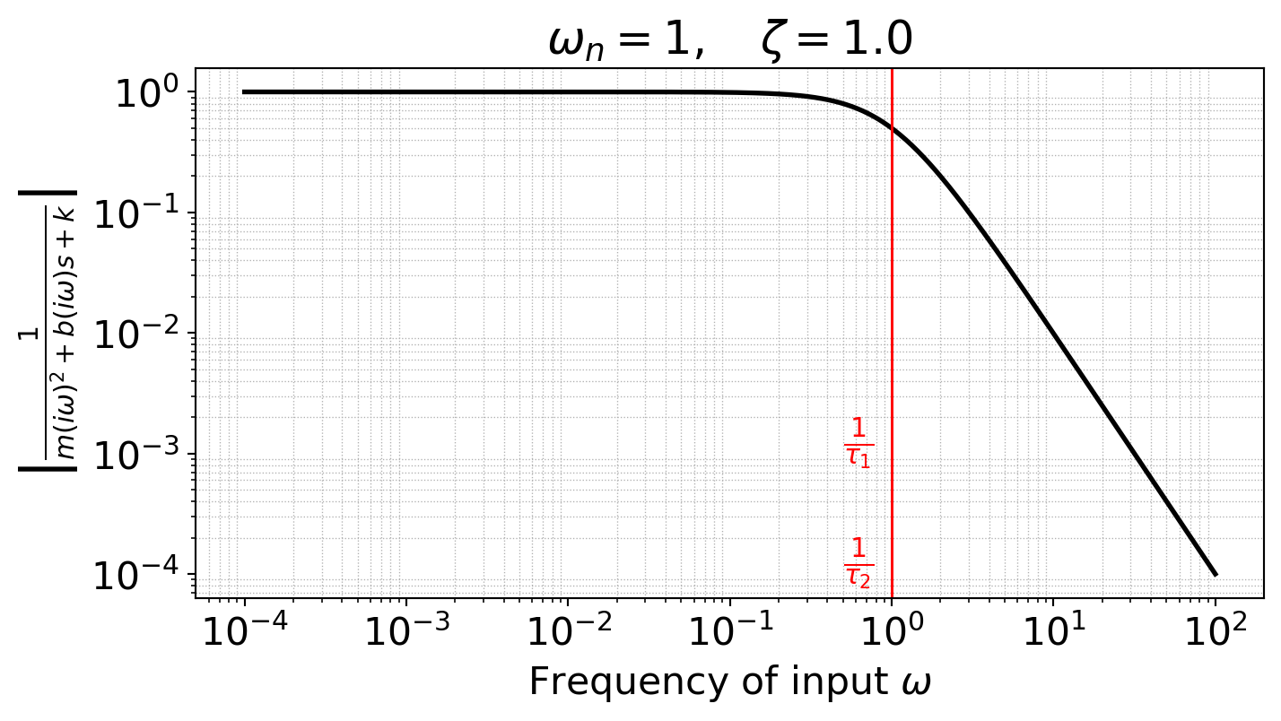
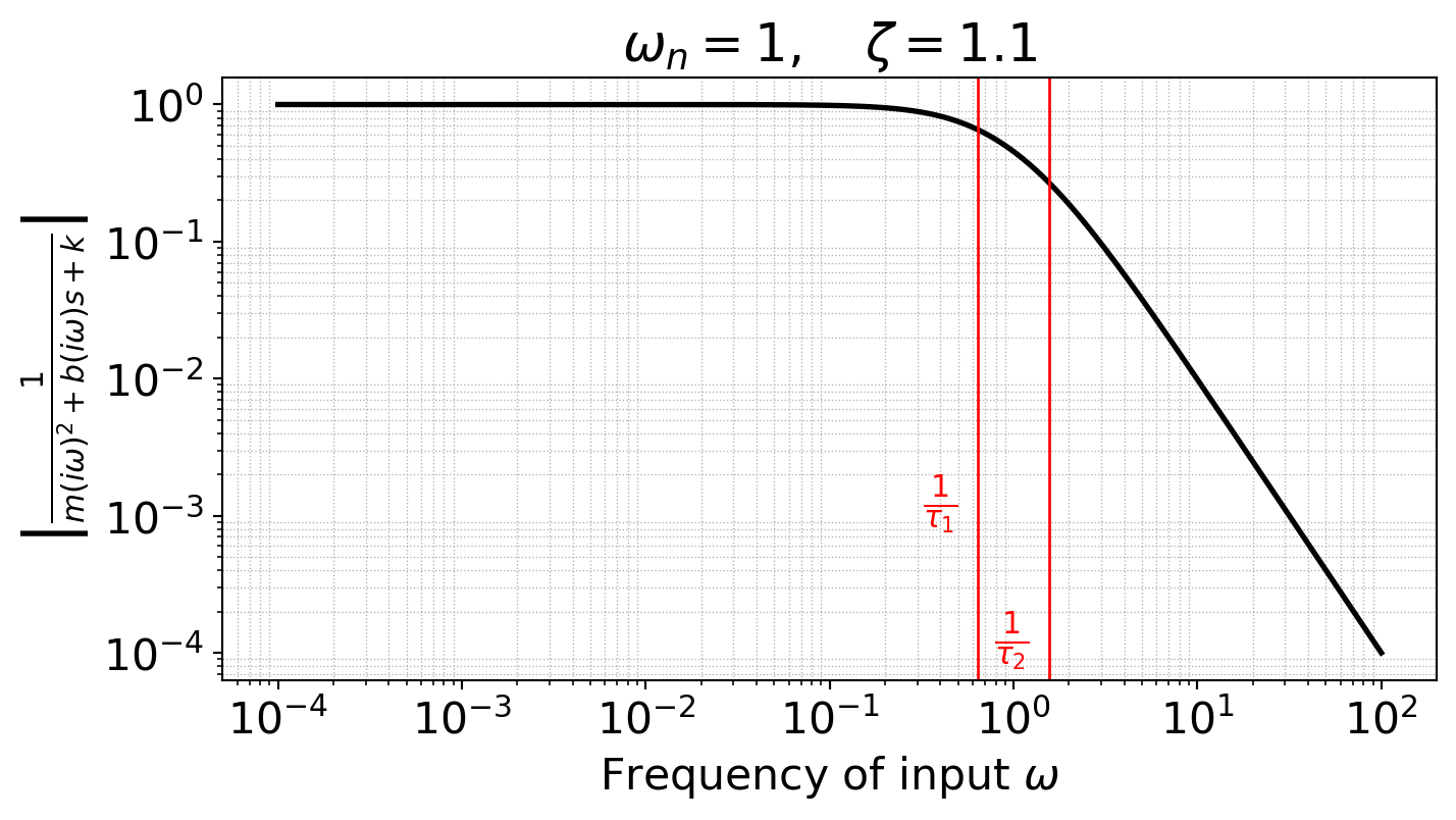
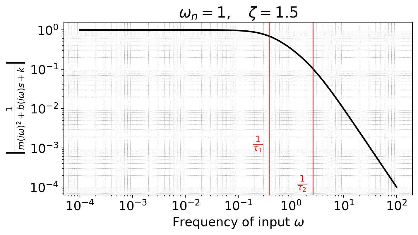
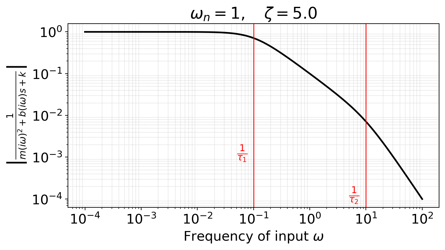
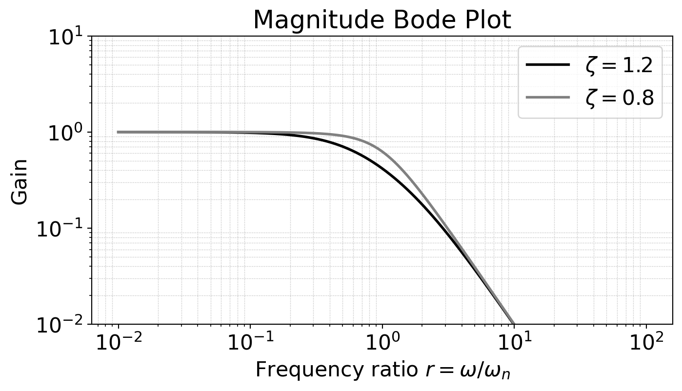
Bode Plots for overdamped systems
Setting \(m = k = 1\) and varying only \(b\) in the range such that \(\zeta >= 1\):
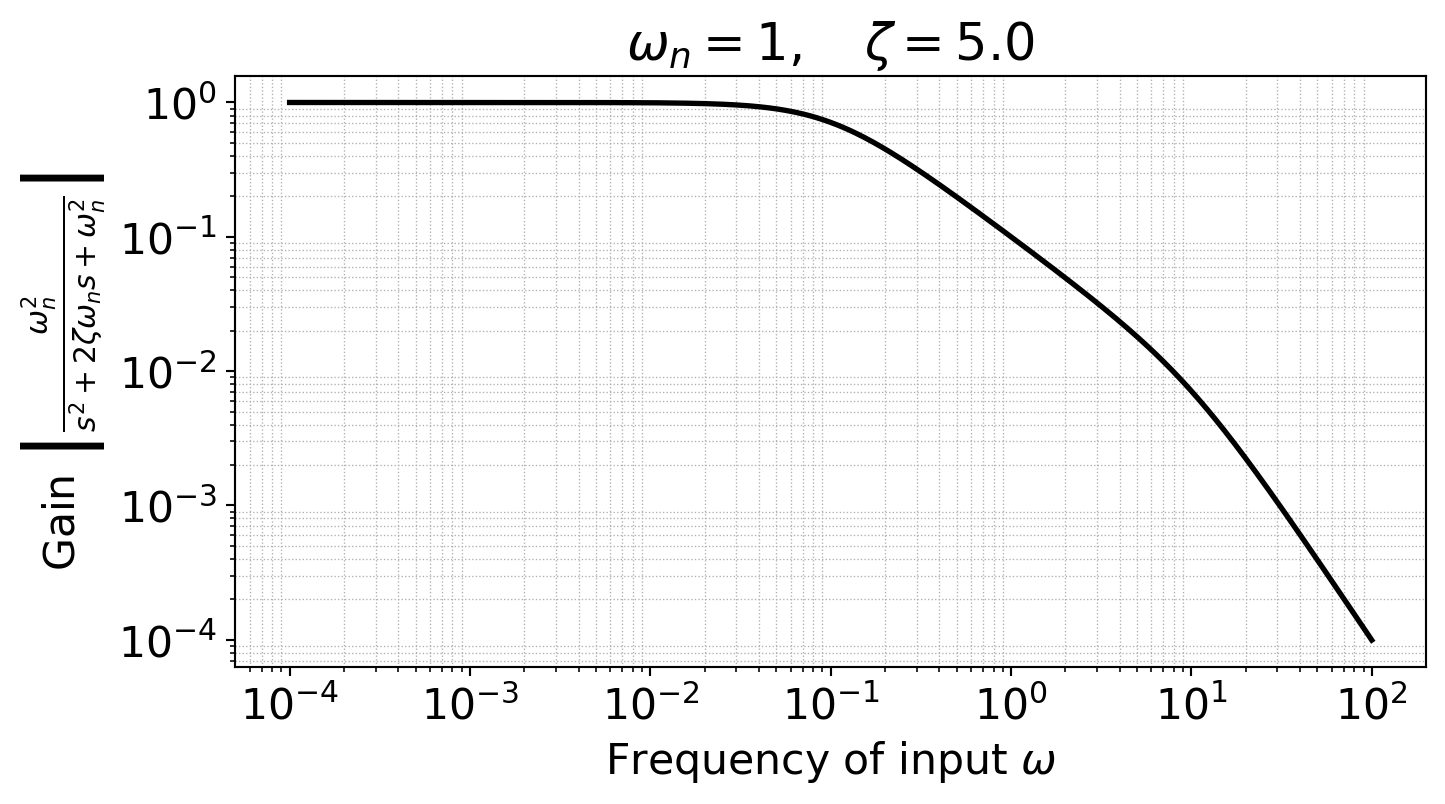
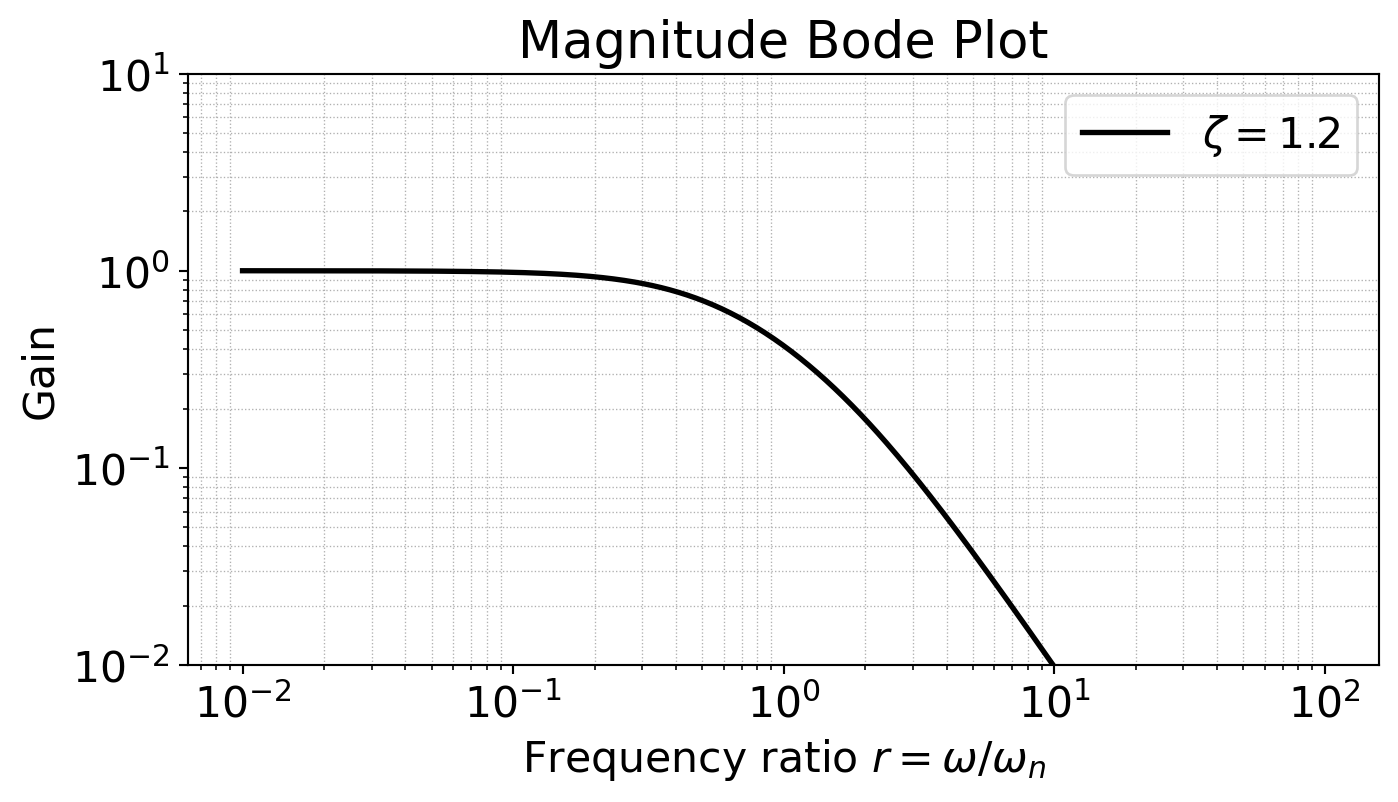
Bode plot as a function of frequency ratio
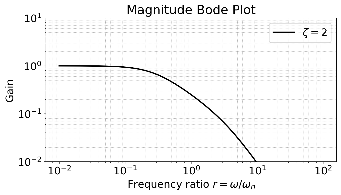
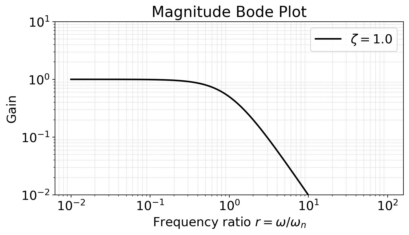
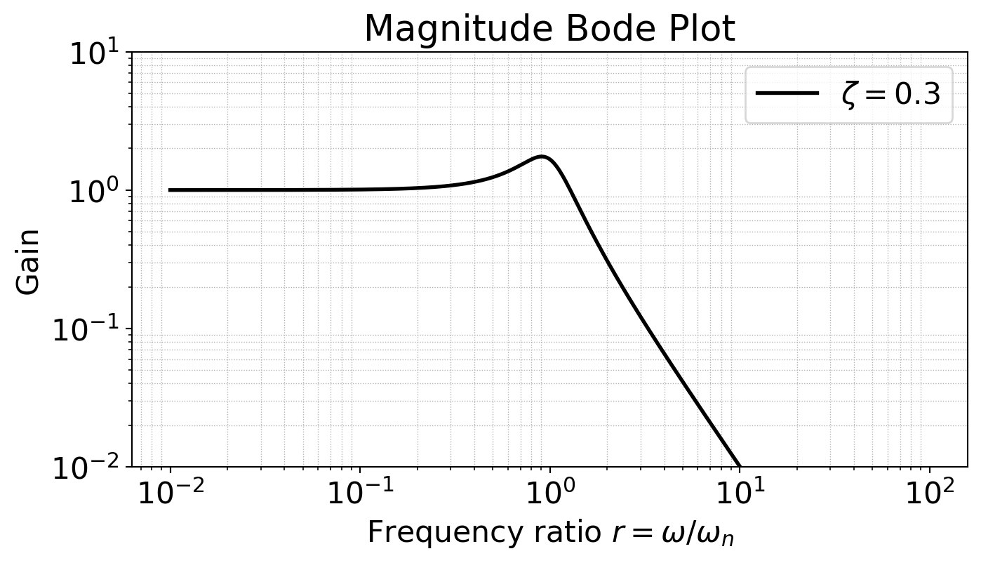
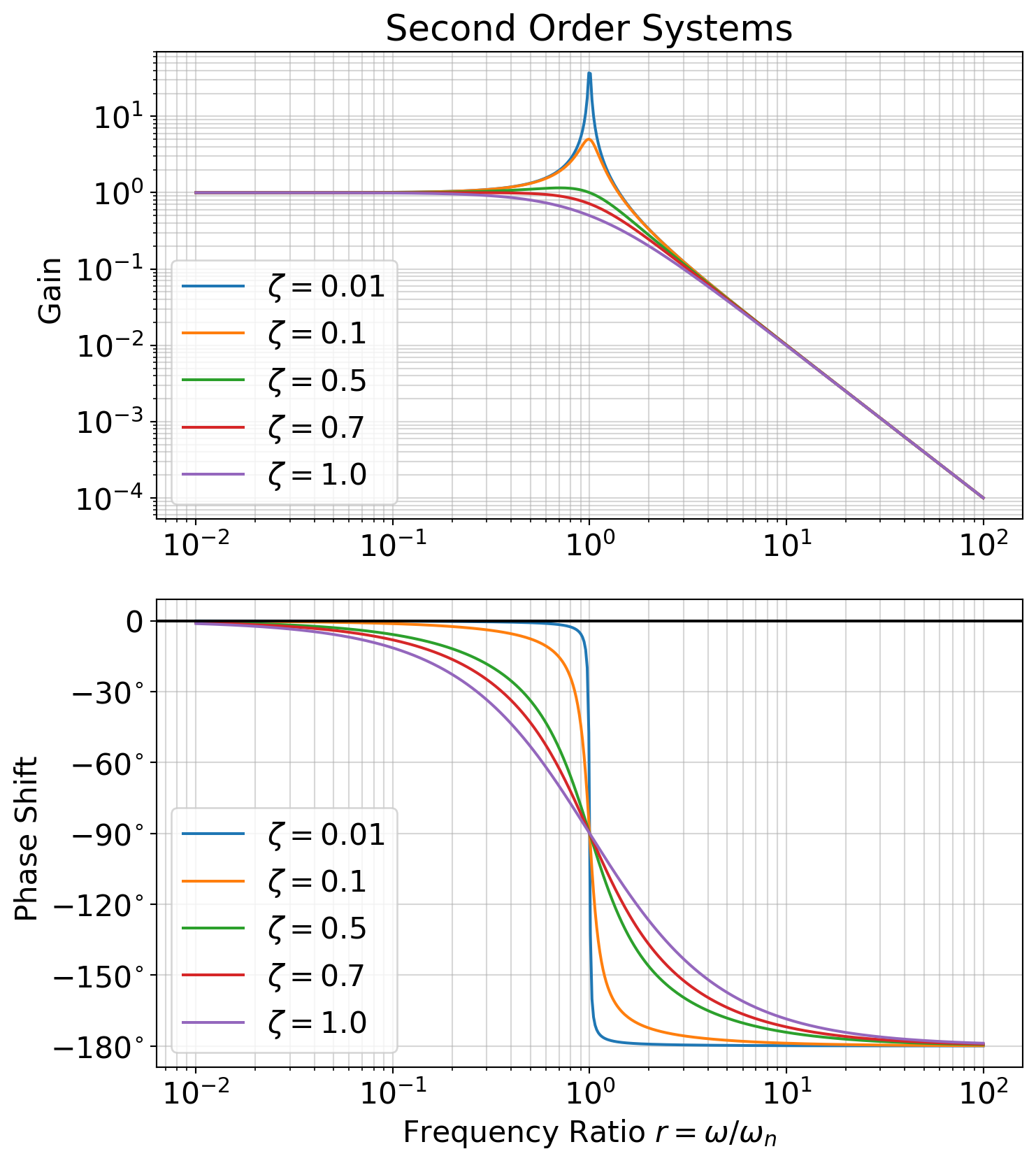
The (magnitude) Bode plot for a 2nd order system \(T(s) = \frac{\omega_n^2}{s^2 + 2 \zeta \omega_n s + \omega_n^2}\) can therefore be represented as \[|T(i \omega)| = \frac{1}{\sqrt{(1-r^2)^2 + 4 \zeta^2 r^2}}\]
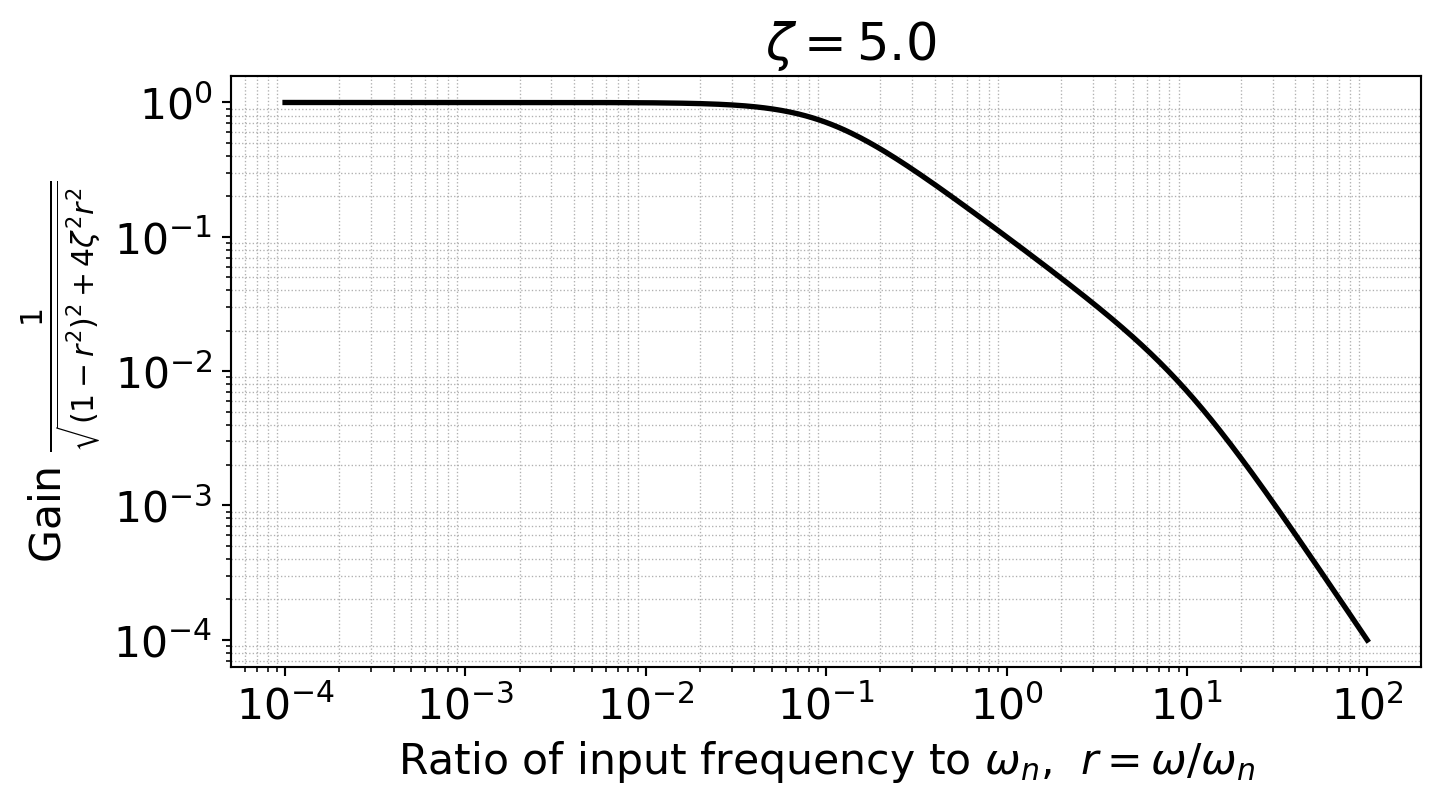
- In this form, the Bode plot has \(r\) on the horizontal axis, gain on the vertical axis, and a single parameter \(\zeta\).
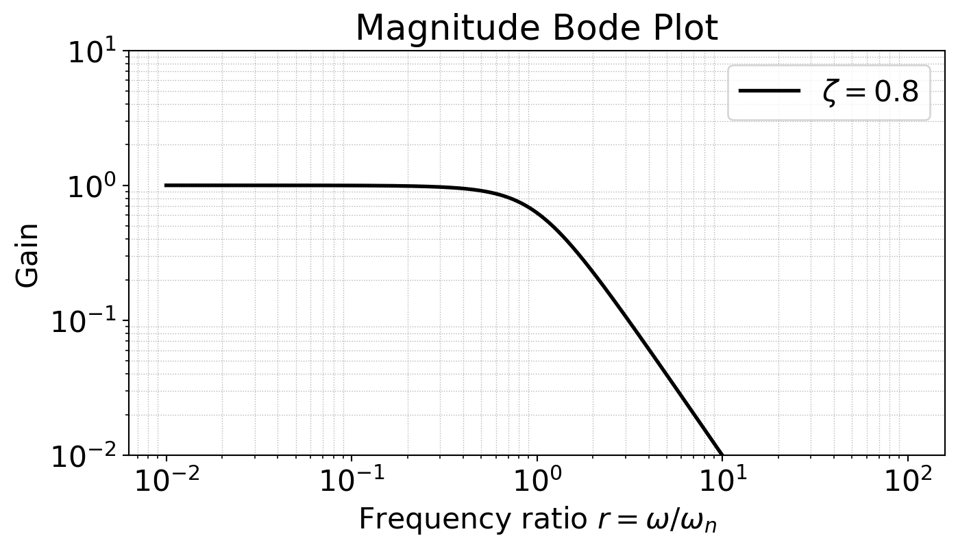
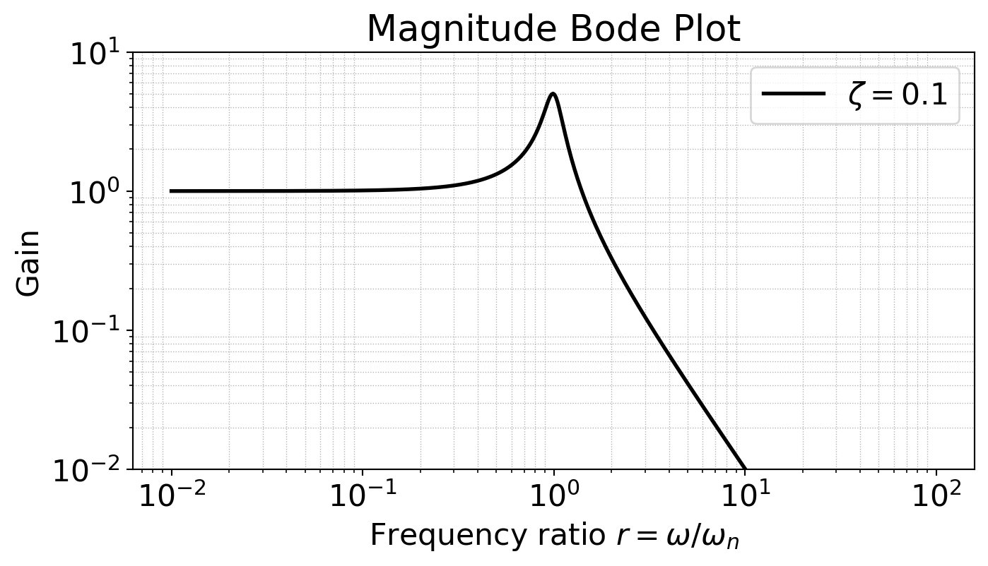
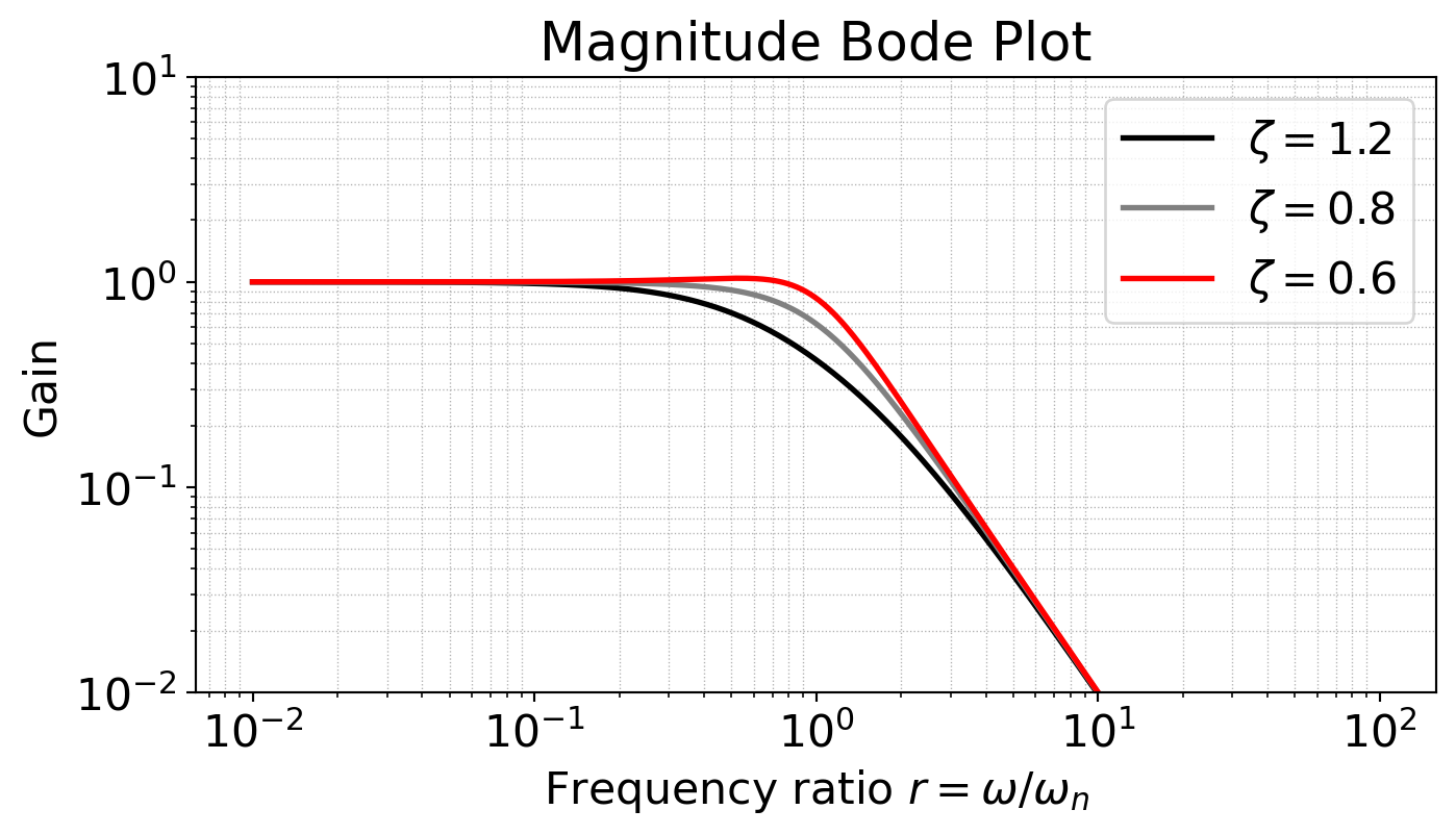
Examples of 2nd order Bode Plots
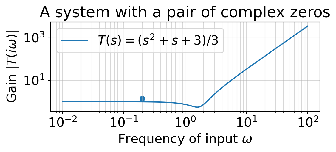
Complex Zeros of the Transfer function
- If a system has complex zeros, then its Bode plot looks similar to the case when it has complex poles, except that it is flipped upside down.
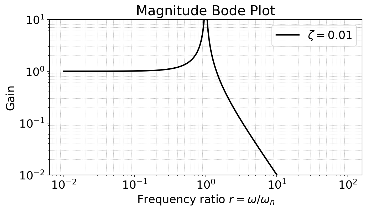
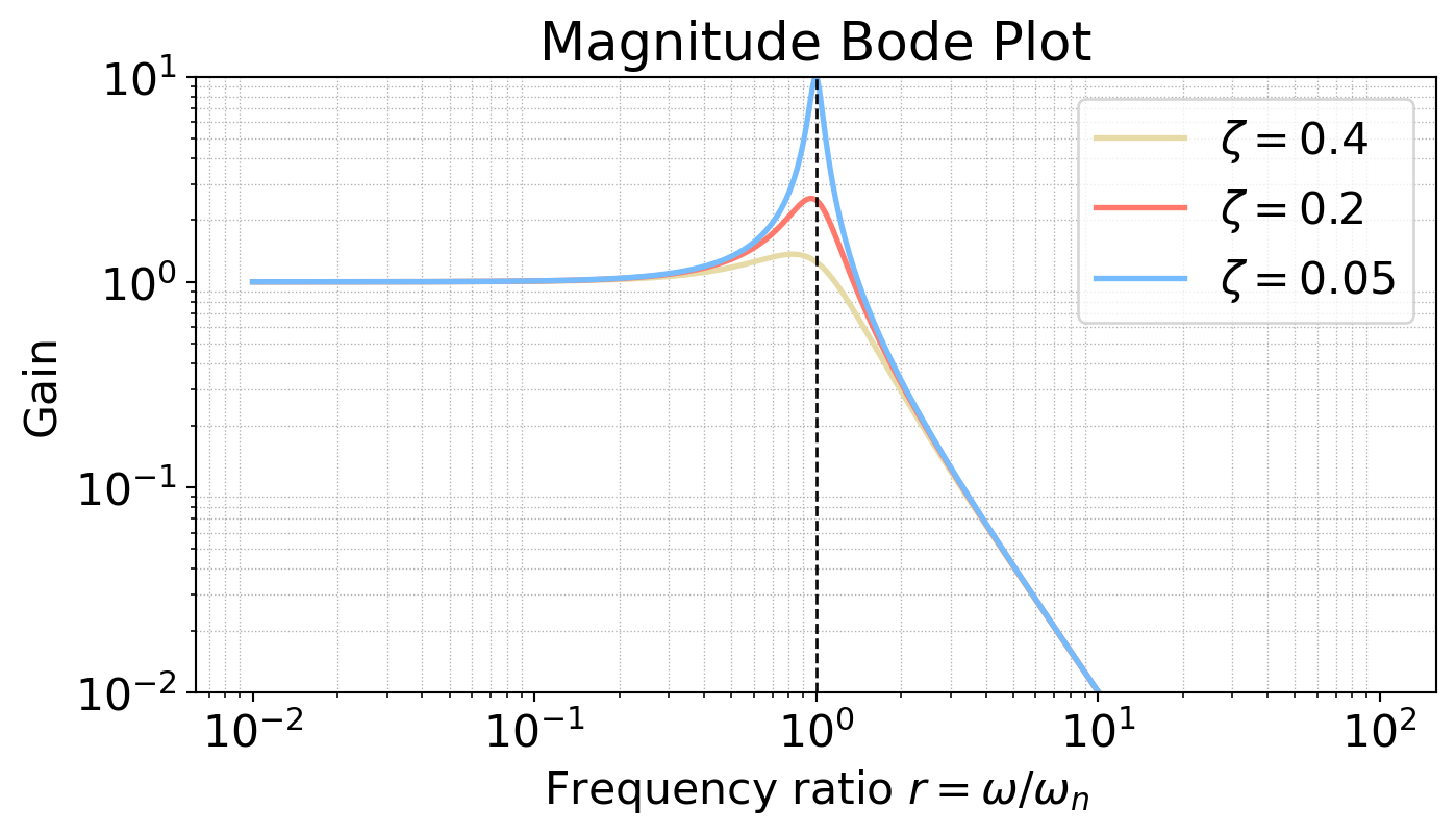
What happens at v. low \(\zeta\)
Let’s zoom in to the Bode plot at small damping ratios.
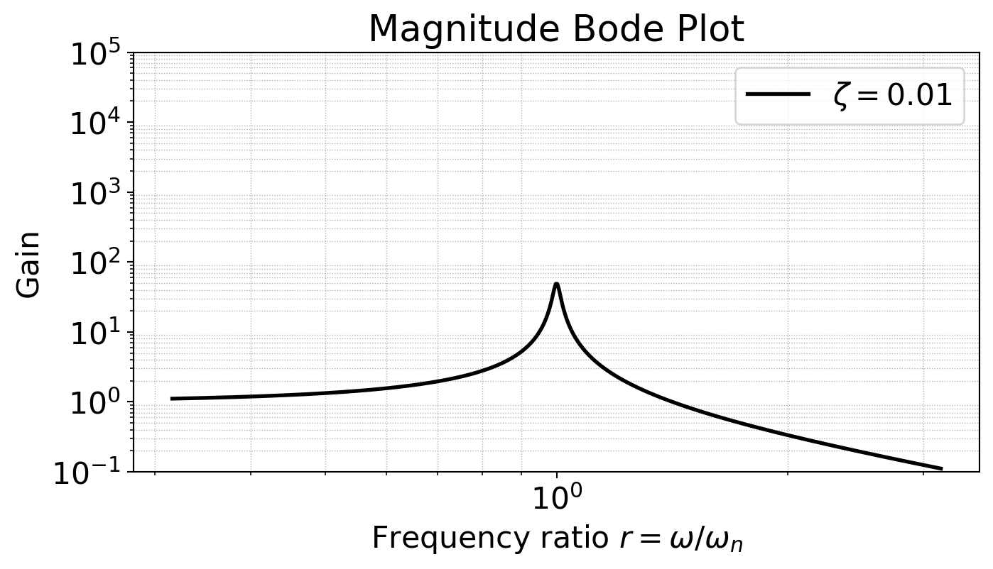
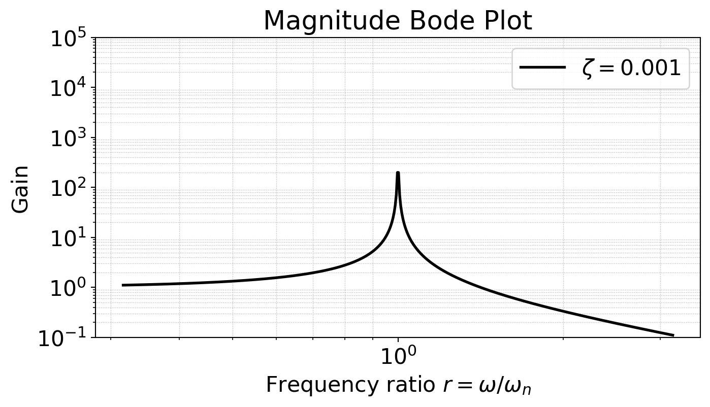
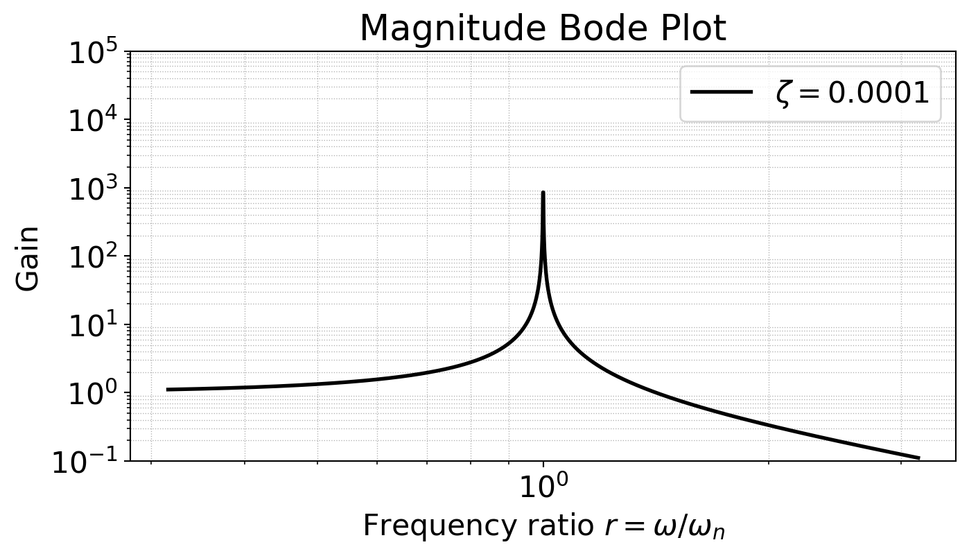
Resonance
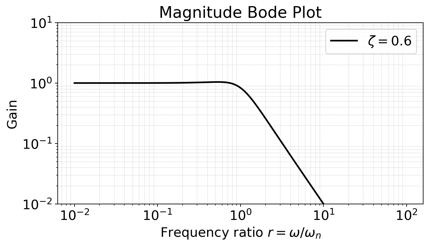
- We notice that there is some critical value of \(\zeta\) below which the Bode plot has a ‘hump’.
- This phenomenon is known as resonance: when the system \(T(s) = \frac{\omega_n^2}{s^2 + 2 \zeta \omega_n s + \omega_n^2}\) has Gain \(>1\).
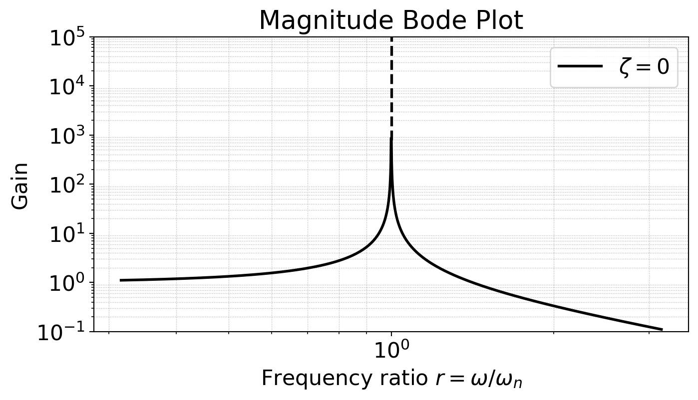
When does resonance happen?
- A maximum in \(\frac{1}{\sqrt{(1-r^2)^2 + 4 \zeta^2 r^2}}\) only occurs when \(r = \sqrt{1 - 2\zeta^2}\)
- If \(\zeta > \frac{\sqrt{2}}{2} \approx 0.707\), resonance does not occur.
- For \(0 < \zeta < \frac{\sqrt{2}}{2}\), the resonant frequency is \[\omega_r = \omega_n \sqrt{1-2\zeta^2}\]
- If the system is excited at this frequency, it will experience resonance.
- The resonant gain \(T(i \omega_r)\) can be shown to be \[|T(i \omega_r)| = \frac{1}{2 \zeta \sqrt{1- \zeta^2}}\]
Comprehensive Bode Plot for second-order systems
In-class activity
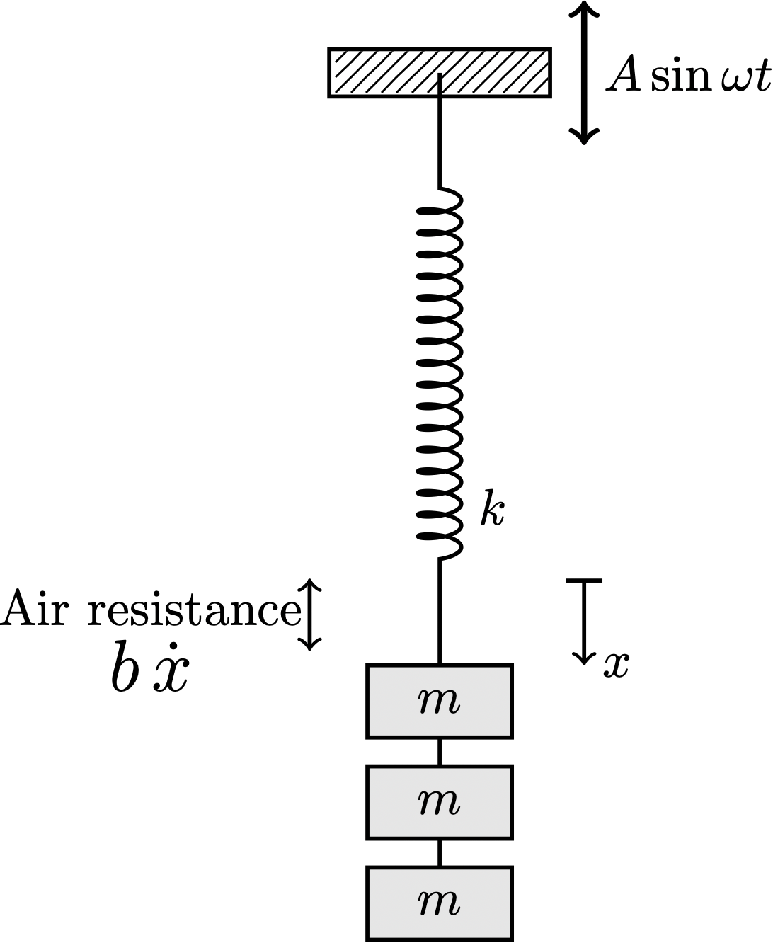
Predict the frequency with which the spring-mass system from Tuesday’s class should be oscillated to achieve resonance. Give your answer in Hertz.
Note that each mass was 200 grams, and the spring is listed as having a spring constant of \(0.2~\mathrm{lbf}/\mathrm{in}\).