Lecture 9

E12 Linear Physical Systems Analysis

Prof. Emad Masroor

February 17, 2026

Second-order Differential Equations

So far, we have looked at (linear) differential equations of the form \[ \dot{x} + ax = f(t), \quad \text{or} \quad \dot{x} = \underbrace{g(t,x)}_{\text{Linear in }x} \quad \text{ with } a > 0 \]

• We now turn to equations of the form \[ \ddot{x} + b \dot{x} + a x = f(t), \quad \text{or} \quad \ddot{x} = \underbrace{g(t,x,\dot{x})}_{\text{Linear in }x\text{ and }\dot{x}} \quad \text{ with } a,b > 0 \]

For simplicity, let’s start with \[ \boxed{\ddot{x} + ax = f(t)}, \quad \text{ with } a > 0 \]

Recall from Lecture 3 that we need two initial conditions now. \(\boxed{x(0) = \text{ some value}}\) & \(\boxed{\dot{x}(0) = \text{some other value}}\)

Physical Motivation: Spring-Mass System

The differential equation \[m\ddot{x} + kx = f(t)\] is a model for the following physical system:

How did we solve 1st-order Differential Equations?

Given \[\frac{dx}{dt} + ax = f(t)\] Separate \(x\) and \(t\) if possible. Integrate. e.g.: \[ \begin{aligned} \frac{dx}{dt} + ax &= 3 \\ \int \frac{dx}{3-ax} &= \int dt \\ \frac{1}{-a}\log (3-ax) &= t + k \\ \log (3-ax) &= -at + k_2 \\ e^{\log (3-ax)} &= e^{-at + k_2} \\ 3-ax &= k_3 e^{-at} \\ & ... \end{aligned} \]

Another approach: ‘Guess’

• Look closely at \[\dot{x} + ax = 0 \tag{1}\]
• “The first derivative of \(x(t)\)” is proportional to \(x(t)\).
• What functions have this property?
  • Is the derivative of \(2t\) proportional to \(2t\)? no
  • Is the derivative of \(\cos 2t\) proportional to \(\cos 2t\)? no
  • Is the derivative of \(\log 2t\) proportional to \(\log 2t\) ? no
  • Is the derivative of \(e^{2t}\) proportional to \(e^{2t}\)? YES
• Plug \(e^{\lambda t}\) into Equation 1 \[ \lambda e^{\lambda t} + a e^{\lambda t} = 0 \implies (\lambda + a) e^{\lambda t} = 0 \]
  • So if \(\lambda = -a\), then \(\boxed{e^{\lambda t}}\) is a solution!

Guessing a solution to second-order equations

• Look closely at \[\ddot{x} + ax = 0 \tag{2}\]
• “The second derivative of \(x(t)\)” is proportional to \(x(t)\).
• What functions have this property?
  • Is the 2nd derivative of \(2t^3\) proportional to \(2t^3\)? no
  • Is the 2nd derivative of \(\log 2t\) proportional to \(\log 2t\) ? no
  • Is the 2nd derivative of \(\cos 2t\) proportional to \(\cos 2t\)? YES
• Plug \(\cos \omega t\) into Equation 2 \[ x(t) = \cos \omega t \implies \dot{x}(t) = - \omega \sin \omega t \implies \ddot{x}(t) = - \omega^2 \cos \omega t \] \[ -\omega^2 \cos \omega t + a \cos \omega t= 0 \implies (- \omega^2 + a) \cos \omega t = 0 \]
  • So if \(\omega^2 = a,\) \(\boxed{\cos \omega t}\) is a solution!

Sines and Cosines solve \(\ddot{x} + ax = 0\)

• The same argument applies to both \(\sin \omega t\) and \(\cos \omega t\).

• Try \(x_1(t) = \cos \omega t\)
• Then \(\ddot{x}_1 = -\omega^2 \cos \omega t\)
• Does it satisfy \(\ddot{x}_1 + ax_1 = 0\) ? \[(-\omega^2+a) \cos \omega t = 0\]
  • YES, if \(\omega^2 = a\)

• Try \(x_2(t) = \sin \omega t\)
• Then \(\ddot{x}_2 = -\omega^2 \sin \omega t\)
• Does it satisfy \(\ddot{x}_2 + ax_2 = 0\) ? \[(-\omega^2+a) \sin \omega t = 0\]
  • YES, if \(\omega^2 = a\)

• Both \(\sin \omega t\) and \(\cos \omega t\) solve \(\ddot{x} + ax = 0\), as long as \(\omega^2 = a\)

The linearity of \(\ddot{x} + ax = 0\)

\[\ddot{x} + ax = 0\]

• If a function \(x_1(t)\) solves Equation 2 and another function \(x_2(t)\) solves Equation 2 then any linear combination of \(x_1\) and \(x_2\) also solves Equation 2. For example:
  • \(3 x_2(t)\) is a solution.
  • \(2x_1(t) - 3 x_2(t)\) is a solution
  • \(x_1(t) + x_2(t)^2\) is not a solution
  • \(x_1(t) x_2(t)\) is not a solution
• Now that we know that \(\cos \omega t\) and \(\sin \omega t\) are solutions, the solution to Equation 2 can be written as \[A \cos \omega t + B \sin \omega t, \quad \omega^2 = a\] for any \(A\) and \(B\).

A note about the right hand side

If our goal is to solve problems of the kind

Why do we study \[\ddot{x} + ax = 0 \tag{3}\] instead of \[\ddot{x} + ax = f(t) \tag{4}\]

• Answer:
  1. If \(x_3(t)\) is a solution to Equation 3 and \(x_4(t)\) is a solution to Equation 4, then \(x_3(t)+x_4(t)\) is also a solution to Equation 4.
  2. Equation 3 corresponds to the ‘free’ response.

Guessing a solution to \(\ddot{x} + ax = 0\) using exponentials instead

\[\ddot{x} + ax = 0, \qquad a > 0\]

The exponential function \(e^x\) or \(\exp x\) is that unique function whose derivative is equal to itself.

Let’s try \(x_3(t) = e^{\lambda t}\). Is this a solution?

\[\underbrace{e^{\lambda t}}_{x_3(t)}\rightarrow \quad \boxed{d/dt} \quad \rightarrow \underbrace{\lambda e^{\lambda t}}_{\dot{x}_3(t)} \rightarrow \quad \boxed{d/dt} \quad \rightarrow \underbrace{\lambda^2 e^{\lambda t}}_{\ddot{x}_3(t)}\]

Now plug \(x_3(t)\) into Equation 2 and check \[ \begin{aligned} \ddot{x}_3 + ax_3 &= 0 \\ \lambda^2 e^{\lambda t} + a e^{\lambda t} &= 0 \\ {(\lambda^2 + a)} e^{\lambda t} &= 0 \end{aligned} \] - This is only zero if \(\lambda^2 +a = 0\), but \(a>0\). uh-oh.

What to do with \(\lambda^2 + a = 0\) when \(a>0\)

There are no real values of \(\lambda\) that solve the equation \(\lambda^2 + a = 0\) when \(a>0\)

But there are imaginary ones!

• Let \(\lambda = +i \omega\) and \(\lambda = - i \omega\) with \(\omega \in \mathbb{R}\). Then \[ (i \omega)^2 + a = i^2 \omega^2 +a = - \omega^2 + a \] and this is zero when \(\omega^2 = a, \omega = \pm \sqrt{a}\)

• Similarly \[ (-i \omega)^2 + a = (-1)^2 i^2 \omega^2 +a = - \omega^2 + a \] and this is zero when \(\omega^2 = a, \omega = \pm \sqrt{a}\)

So \(\lambda = \pm i \omega, \, \omega \in \mathbb{R}\) is a solution to \(\lambda^2 + a = 0\)

Exponential solutions to \(\ddot{x} + ax = 0\)

To summarize,

\(x(t) = e^{\lambda t}\) is a solution to Equation 2 if \[\lambda = \pm i \omega, \quad \omega^2 = a, \quad a,\omega > 0\]

\[\boxed{x(t) = e^{\pm i \omega t}}\]

Equivalence of the trigonometric and exponential solutions

Forms of the solution to \(\ddot{x} + ax = 0, a > 0\)

• Sum of cosines and sines with \(A,B \in \mathbb{R}\) \[x(t) = A \cos \omega t + B \sin \omega t\]
• Complex Exponentials with real coefficients \(C,D \in \mathbb{R}\) \[x(t) = C e^{i\omega t} + D e^{-i \omega t}\]
  • Must take the real (or imaginary) part if real solutions are desired.
• Complex Exponentials with complex coefficients \(P \in \mathbb{C}\): \[x(t) = P e^{i \omega t} + \overline{P} e^{-i \omega t}\]
  • \(\displaystyle P = \frac{A}{2} + \frac{B}{2i}\) and \(\displaystyle \overline{P} = \frac{A}{2} - \frac{B}{2i}\)
  • No need to take real/imaginary part
• Complex Exponentials with complex coefficients \(Q,R \in \mathbb{C}\): \[x(t) = Q e^{i \omega t} + R e^{-i \omega t}\]
  • Must take the real (or imaginary) part if real solutions are desired.
• Shifted Cosine \(F \in \mathbb{R}\): \(\displaystyle x(t) = F \cos (\omega t + \phi_1), \quad \phi_1 \in [0,2\pi)\)
• Shifted Sine \(G \in \mathbb{R}\): \(\displaystyle x(t) = G \sin (\omega t + \phi_2), \quad \phi_2 \in [0,2\pi)\)

for any real numbers \(A\), \(B\), \(C\), \(D\), \(F\), \(G\) and any complex numbers \(P\), \(Q\) and \(R\).

Initial Value Problem

Solve the differential equation \[\ddot{x} + ax = 0, \quad a > 0 \] subject to the initial condition on position \[x(0) = x_0\] and the initial condition on velocity \[\dot{x}(0) = v_0\] using the trigonometric ‘guess’ \(x(t) = A \cos \omega t + B \sin \omega t\)

• Solution: \[ \begin{aligned} x(t) = x_0 \cos \omega t + \frac{v_0}{\omega} \sin \omega t, \end{aligned} \] where \(\omega^2 = a\)

A spring-mass system released from rest

Solve the differential equation \[\ddot{x} + ax = 0, \quad a > 0 \] subject to the initial condition on position \[x(0) = 1.0\] and the initial condition on velocity \[\dot{x}(0) = 0.0\]

A spring-mass system released at speed

Solve the differential equation \[\ddot{x} + ax = 0, \quad a > 0 \] subject to the initial condition on position \[x(0) = 0.0\] and the initial condition on velocity \[\dot{x}(0) = 1.0\]

Compare initial \(x(0)\) with initial \(\dot{x}(0)\)

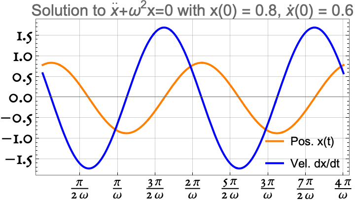
A spring-mass system released with nonzero position and velocity

Solve the differential equation \[\ddot{x} + ax = 0, \quad a > 0 \] subject to the initial condition on position \[x(0) \neq 0\] and the initial condition on velocity \[\dot{x}(0) \neq 0\]

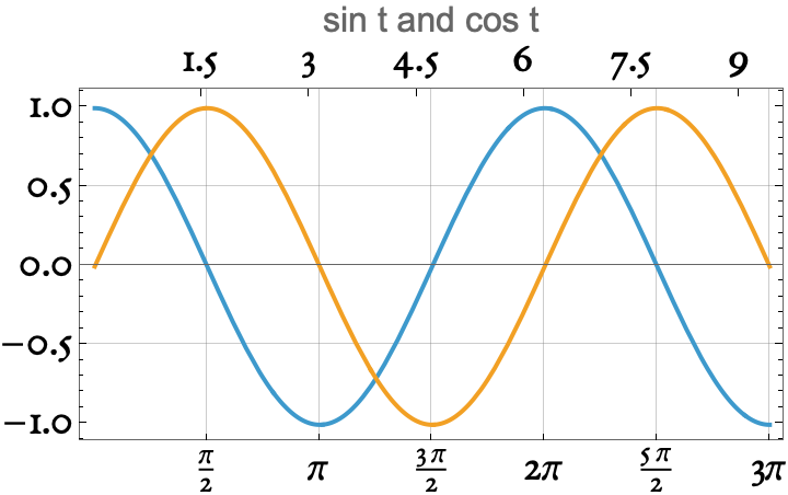
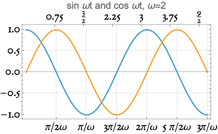
Recall some features of sine and cosine

• The period of \(\cos \omega t\) and of \(\sin \omega t\) is \(2\pi/\omega\) seconds
• When \(\cos \omega t\) is at zero, \(|\sin \omega t |\) is at a maximum
• When \(\sin \omega t\) is at zero, \(|\cos \omega t |\) is at a maximum
• \(\cos \omega t\) is (a constant times) the derivative of \(\sin \omega t\) with respect to \(t\)
• \(\cos \omega t\) is a phase-shifted version of \(\sin \omega t\)

A closer look at the solution