Lab 3: Stiffness of Beams under Bending
ENGR 059 • Fall 2026 • Swarthmore Engineering
In the online version of this document, the pointed hand symbol (☞) draws your attention to required tasks.
1 Background and Theory
1.1 Three-point Bending
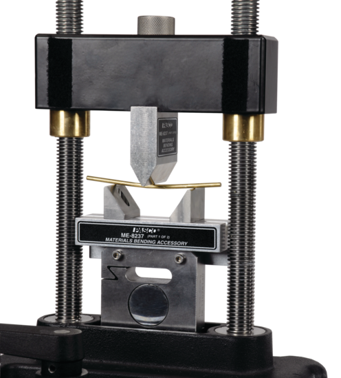
3-point bending refers to a method of loading a beam in which transverse force is applied to the beam at three locations. A general schematic is shown below.
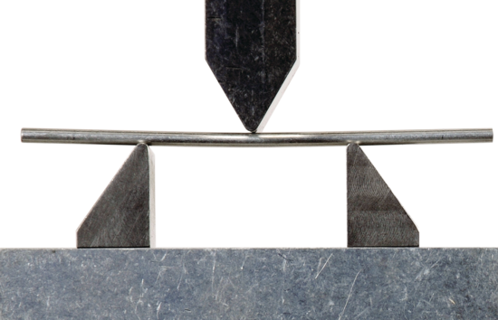
Under small loads of this type, beams show elastic behavior. In this lab, you will characterize this elastic behaviour of beams under 3-point loading.
1.2 Shear, Moment, Slope and Deflection curves for pure 3-point bending
Pure 3-point bending refers to a loading arrangement as shown in Figure 1, where the loads are applied exactly at the endpoints of the beam.
The quantities
- shear, \(V(x)\), in Newtons,
- moment \(M(x)\), in Newton-meters,
- slope, \(\theta(x)\) (or \(y'(x)\)), unitless, and
- deflection, \(y(x)\), in meters,
are related to each other by the following equations.
\[\frac{dM}{dx} = V(x) \tag{1}\] \[EI \frac{d^2 y}{d x^2} = M(x) \tag{2}\]
where \(E\) is the Young’s modulus of the given beam’s material and \(I\) the second moment of the area of the beam’s cross-sectional shape. Multiplied together, the quantity \(EI\) is known as the flexeural rigidity of a beam and is affected by both the shape and the material of the beam.
For pure three-point bending in which the loads are applied as shown in Figure 1,
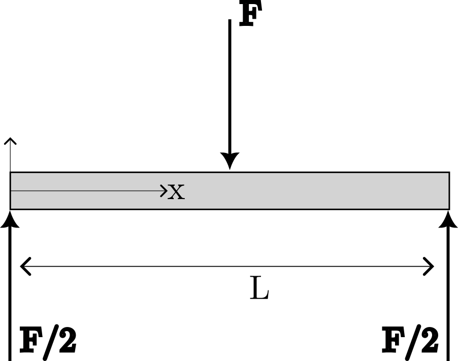
the shear, moment, slope and deflection curves are shown in Figure 2.
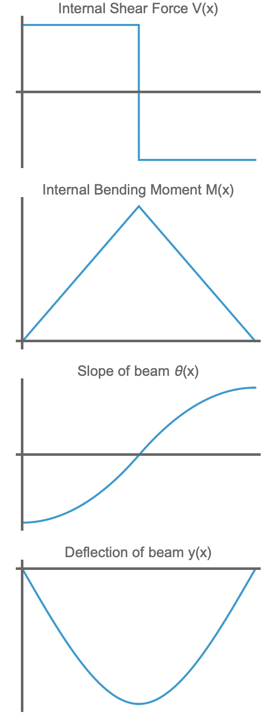
The curves in Figure 2 can be derived by noting that the shear force inside the beam is
\[V(x) = \begin{cases} +F/2 \quad 0 < x < L/2 \\ -F/2 \quad L/2 < x < L \end{cases} \]
The bending moment can be found with the help of Equation 1, noting that the loading anvil acts as a pin/roller support with no moment.
The slope can be found by integrating the bending moment \(M(x)\) with respect to \(x\); it may be assumed by symmetry that the slope of the beam is zero degrees at the center where \(x/L = 1/2\).
Finally, the deflection of the beam \(y(x)\) can be found by integrating the slope with respect to \(x\) and using the boundary condition that \(y=0\) at the bottom support \(x=0\).
1.3 Second Moment of the Area
The second moment of an area about an axis, also known as the ‘moment of inertia’, is a measure of how much a given area is distributed around an axis, versus being concentrated near it. For a rectangle, the moment of inertia about its centroidal axis is given by \[I = \frac{1}{12} b h^3,\] where \(h\) is the side of the rectangle that is aligned with the load vector.
Note that Mode 1 (Figure 4) and Mode 2 (Figure 5) of loading will have different values of \(I\).
1.4 Stress
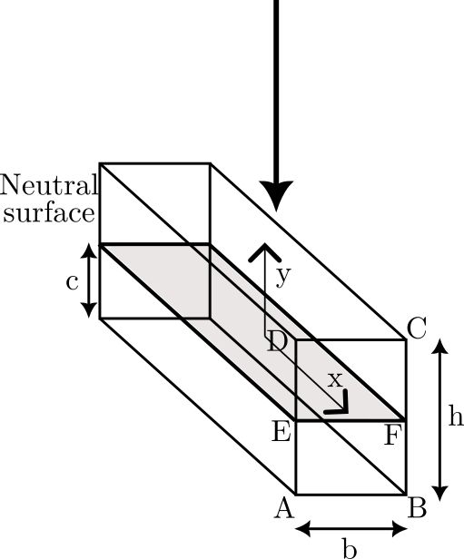
The normal stress due to bending is directly proportional to the bending moment \(M\), and is given by \[\sigma = -\frac{M y}{I},\] where \(y\) is to be interpreted as shown in Figure 3 and \(I\) is the second moment of the cross-sectional area ABCD about the neutral axis EF.
1.4.1 ☞ Calculate expected maximum stress
Use a back-of-the-envelope calculation to determine the expected normal stress in the beam (in MPa) depending on the value of \(F\) (in Newtons), the load applied by the Materials Testing System.
Using this calculation, decide on a value of \(F\) which you will not exceed in the parts of this lab that require you to remain within the elastic region. You should get this calculation checked by the instructor before proceeding with Section 3.4
1.5 ☞ Maximum Deflection
It can be seen from Figure 2 that the deflection of the beam will be greatest at its midpoint. This deflection is known from linear elastic beam bending theory to be equal to \[y_{\text{max}} = - \boxed{?} \frac{F L^3}{E I}\, , \tag{3}\]
where \(\boxed{?}\) is a number to be found theoretically.
1.6 ☞ ‘Spring Constant’ of a beam
If a beam deflects by \(y_{\text{max}}\) when loaded with a force \(F\), it is possible to interpret this as a ‘spring constant’ \(k\). Using the relation \[\frac{\text{Force}}{\text{Deflection}} = \text{Spring constant }k \, ,\] we learn that the ‘spring constant’ for a beam under pure 3-point bending load is \[k = \frac{E I}{\boxed{?} L^3}. \tag{4}\]
2 Equipment
Aluminum samples are made of 6065-T6 alloy.
2.1 Samples
2.1.1 Modes of loading the beam
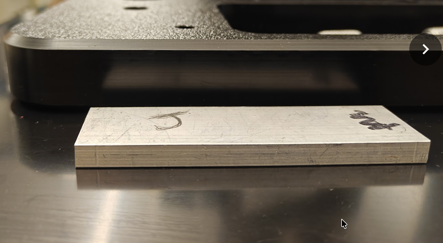
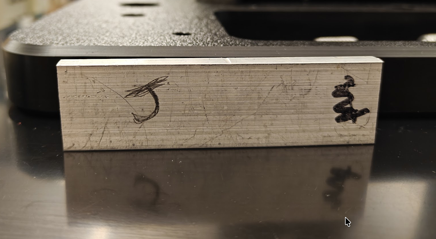
There are two different ways of loading the beam, illustrated in Figure 4 and Figure 5. In Mode 1, the beam is kept on its flat side. In Mode 2, the beam is kept on its narrow side.
2.1.2 Symmetric Loading and Value of \(\eta\)
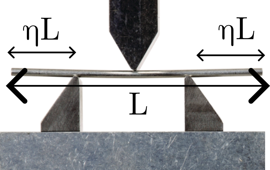
The parameter \(\eta\), illustrated in Figure 6, measures how much room you leave on either side of the edge of the beam. You will always load the beam symmetrically.
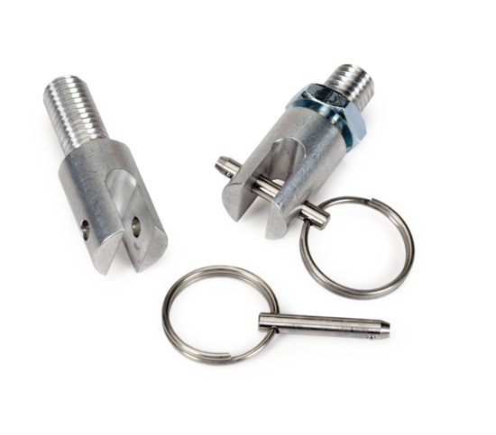
2.2 Attachments to ME-8236
3 Experimental Tasks
3.1 ☞ Warm-up with spring
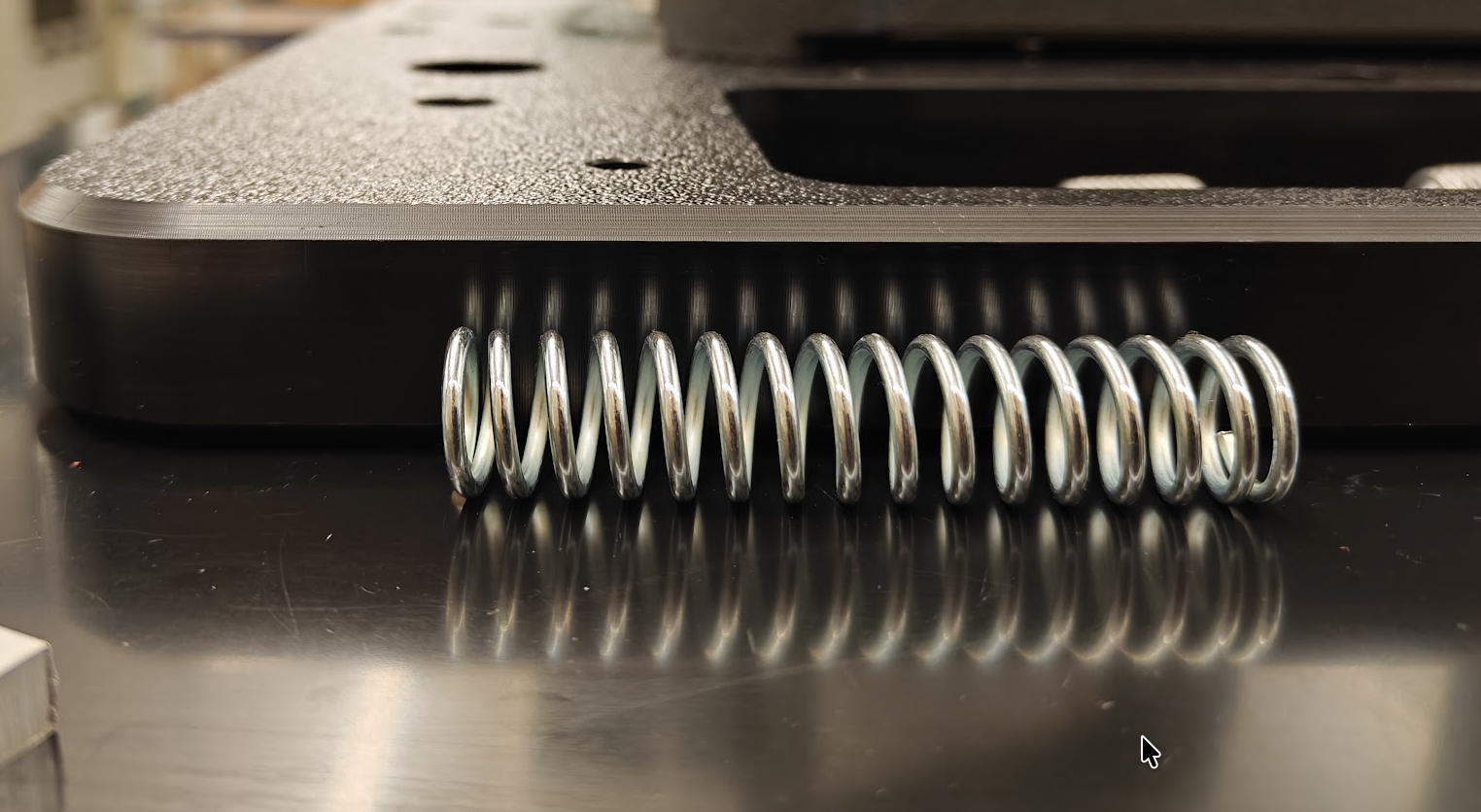
Use the Materials Testing Machine together with the clevis fastener (Figure 7) to generate a force-deflection curve for the given spring. A single load-unload cycle is sufficient for this. Make sure you determine a satisfactory estimate of the spring constant \(k\) before proceeding. If the spring is stretched into its plastic regime in the course of testing, that’s okay.
It is not necessary to calibrate the machine for this purpose.
3.2 ☞ Calibration
Calibrate the materials testing system in compression up to the maximum number of Newtons that you intend to apply to the samples.
3.3 ☞ Three-point loading to failure
Load one specimen of the beam to failure in either Mode 1 or Mode 2 using \(\eta \approx 0\) if possible. Record force, position, and time data. Maintain a low speed of advancement.
Do not exceed 7,000 N of force or you will damage the load cell.
3.4 ☞ Elastic behavior of beam
For this part, use the same mode of loading as you did for Section 3.3.
Apply a 3-point bending load to the beam using 10 different values of \(\eta\), starting from the smallest value (\(\eta \rightarrow 0\)) and working your way up to a large fraction in small increments. For each test, load and unload the beam slowly.
You must attempt to keep the beam in an elastic regime. It should be safe to load the beam up to 4,000 N.
The highest theoretically possible value is \(\eta = 1/2\), but there may be technical limitations to achieving a number close to this value. Plan out approximately what values of \(\eta\) you will aim for, and record actual measurements of how you positioned the beam relative to the anvils to calculate a precise value of \(\eta\) each time.
Make a table with columns showing the value of \(\eta\) you used and the value of the spring constant \(k\) that was determined, for each of your ten data sets.
4 ☞ Extension of Theory
Recall that the formulae Equation 3 and Equation 4 assume pure 3-point bending where \(\eta = 0\). As part of this lab, you must derive a formula for \(y_{\text{max}}\) when 3-point loading is applied with a nonzero value of \(\eta\). As a hint, Figure 8 shows the shear, moment, slope, and deflection of a beam undergoing 3-point bending with \(\eta = 1/4\).
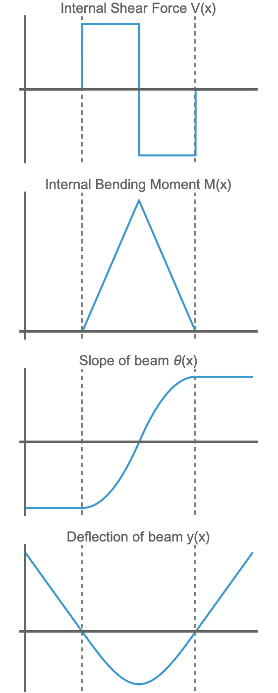
After extending this theory to 3-point bending with nonzero values of \(\eta\), you will find that the maximum deflection is given by \[y_{\text{max}} = - \boxed{?} \frac{F L^3}{EI} \times \text{ some function of }\eta, \tag{5}\] where \(\boxed{?}\) has the same value as in Equation 4. When \(\eta = 0\) is substituted into this formula, you should recover Equation 4 exactly.
The boundary conditions will be slightly different in the case of nonzero \(\eta\) compared with those provided in Section 1.2. While \(\theta(x)\) can still be assumed zero at the midpoint, \(y(x)\) will be zero at \(x/L = \eta\); at \(x=0\) the deflection is certainly not zero.
5 Report
This assignment aims to characterize the elastic behavior of beams under 3-point bending.
Write a lab report describing your efforts to match experimental measurements of a real beam undergoing 3-point bending to the theoretical predictions suggested by what is known as Euler-Bernoulli Beam Theory, which has been summarized in Section 1.
Your report must give adequate space to the derivation of formulae for \(k\) and \(y_{\text{max}}\) for pure 3-point bending, starting from the governing equations Equation 1 and Equation 2. It should then apprise your attempts at determining the value of these quantities from your own experiments.
Furthermore, you should expand the theory to determine a formula for \(y_{\text{max}}\) and \(k\) that is applicable to non-zero values of \(\eta\) as well, completing the unknown parts of Equation 5. Compare your observed values versus this expanded theory.
A suggested set of headings for the sections of your lab report is: Introduction, Theory, Experiments, Conclusion. You do not need a Methods section; where appropriate, methods can be referenced under Experiments.
For an outstanding theory section, provide correct mathematical expressions for \(V(x)\), \(M(x)\), \(\theta(x)\) and \(y(x)\) for one (pure 3-point bending) or both (i.e., pure as well as \(\eta \neq 0\)) types of 3-point bending. These expressions should be symbolic in terms of \(F\), \(L\), \(\eta\), \(E\), \(I\), &c. as appropriate.